What deep learning is, the three learning paradigms, the ethics of deployed systems, and the supervised learning recipe in miniature.
Author
Harun Pirim
Reading Prince, Understanding Deep Learning, Chapter 1 (pp. 1–16) and Chapter 2 (pp. 17–24) · UDL notebook 1.1 (Background mathematics)
Assignment A1 — Foundations
A formative notebook spanning Weeks 1 and 2: the learning paradigms, the supervised recipe, and the Appendix B algebra behind one layer. Every task ends in a self-check that tells you at once whether the idea landed.
In Colab choose File → Save a copy in Drive before you start. When you are done, Runtime → Run all, then File → Download → Download .ipynb and upload that file on Blackboard under Assignment A1, named A1_<lastname>.ipynb. The deadline is posted on Blackboard.
How to read the references in these notes
Every section below opens with the section number and page range it covers in Prince, Understanding Deep Learning (MIT Press, 2024). Page numbers are those of the printed book. Figures taken from the textbook are captioned with their original figure number and page; figures generated by the code in this page are ours. A complete cross-reference table appears in Section 12.
1 Learning Objectives
By the end of this week you should be able to:
Place artificial intelligence, machine learning, deep learning, and deep neural networks in the correct containment relationship.
Distinguish supervised, unsupervised, and reinforcement learning, and classify a new problem into one of them.
Tell regression, multivariate regression, binary classification, and multiclass classification apart from the shape of the output.
Explain what makes an input hard — size, variable length, and internal structure — and why that shapes model design.
Say precisely what a model, its parameters, a loss function, training, and inference are.
Explain what latent variables buy a generative model.
State the temporal credit assignment problem and the exploration–exploitation trade-off.
Discuss the five ethical concerns Prince raises and give a concrete example of each.
Work 1D linear regression end to end: model, loss surface, gradient descent, test error.
The field comes with a stack of terms that get used interchangeably in press coverage and should not be.
Artificial intelligence is concerned with building systems that simulate intelligent behavior. It is a broad church that includes logic, search, and probabilistic reasoning — approaches that involve no learning at all.
Machine learning is the subset of AI that “learns to make decisions by fitting mathematical models to observed data” (p. 1). Prince notes dryly that this area “has seen explosive growth and is now (incorrectly) almost synonymous with the term AI.”
A deep neural network is one particular type of machine learning model.
Deep learning is what we call the act of fitting such a network to data.
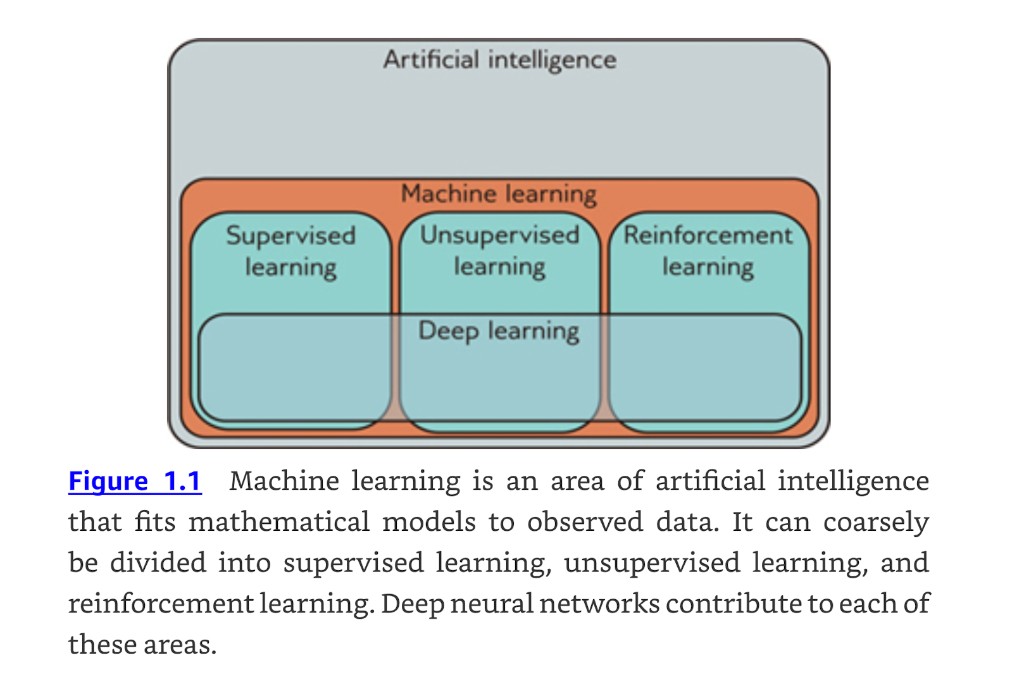
So the containment is strict: deep learning sits inside machine learning, which sits inside artificial intelligence. fig. 1 is the picture to keep in your head for the rest of the semester.
Figure 1: Prince (2024), figure 1.1, p. 2.
Machine learning divides coarsely into three areas — supervised, unsupervised, and reinforcement learning — and, at the time of writing, the leading method in all three is a deep network. That three-way split organizes both the textbook and this course.
What this book is, and is not
Prince describes the book as “neither terribly theoretical (there are no proofs) nor extremely practical (there is almost no code)” (p. 1). The goal is the underlying ideas. These notes add the code back in, because writing the thing down in PyTorch is often what makes the idea stick.
3 Supervised Learning
Prince §1.1, pp. 1–7.
A supervised learning model defines a mapping from input data to an output prediction. That one sentence is the whole definition; the rest of §1.1 asks what the inputs look like, what the outputs look like, what sits in between, and what “training” means.
3.1 Regression and classification
Prince §1.1.1, p. 2; figure on p. 3.
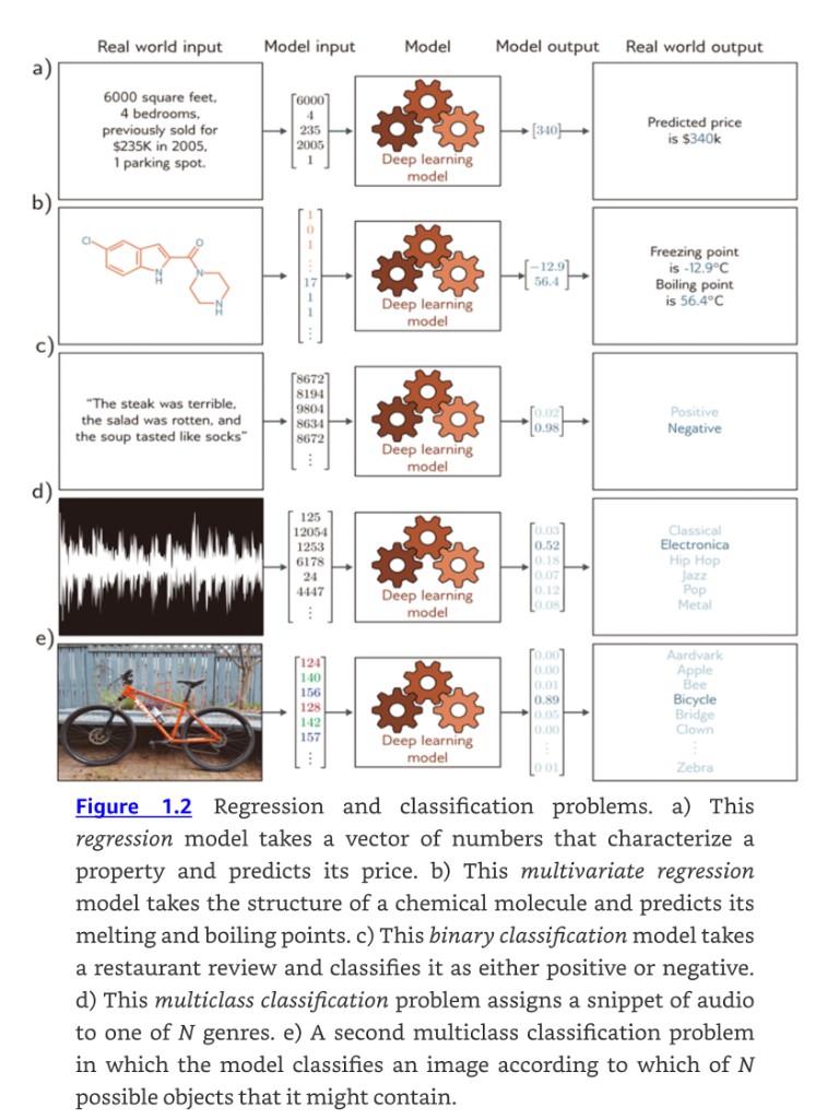
In every supervised problem there is a meaningful real-world input — a sentence, a sound file, an image — which gets encoded as a vector of numbers. That vector is the model input. The model maps it to an output vector, which is then translated back into a meaningful real-world prediction. For now the model is a black box that ingests numbers and returns numbers.
Figure 2: Prince (2024), figure 1.2, p. 3.
The five panels of fig. 2 cover the standard taxonomy. What separates them is entirely the shape and meaning of the output vector:
Melting and boiling point from molecular structure
two continuous numbers
multivariate regression
c
Restaurant review sentiment
probabilities over 2 categories
binary classification
d
Music genre from an audio clip
probabilities over \(N\) categories
multiclass classification
e
Object identity from an image
probabilities over \(N\) categories
multiclass classification
Two things worth pinning down. A regression model returns a continuous number rather than a category assignment; it becomes multivariate regression as soon as it predicts more than one number. A classification model returns a vector of length \(N\) containing the probabilities that the input belongs to each of the \(N\) categories — binary when \(N = 2\), multiclass when \(N > 2\).
3.2 Inputs are the hard part
Prince §1.1.2, pp. 2–4.
The five inputs in fig. 2 look superficially alike once they are vectors, but they differ in ways that will drive every architectural decision in this course.
Tabular data has no internal structure. The house price input is a fixed-length vector of property characteristics. If we permute the entries and retrain, we expect the same predictions. Nothing is lost by scrambling the order.
Text is variable length and order matters. A review may be any number of words long, and, as Prince puts it, “my wife ate the chicken is not the same as the chicken ate my wife.” The text must be encoded numerically first; the book’s running example uses a fixed vocabulary of 10,000 words and simply concatenates the word indices.
Audio is fixed length but enormous. Digital audio is usually sampled at 44.1 kHz with 16-bit integers, so a ten-second clip is 441,000 numbers.
Images are enormous and two-dimensional. The input is the concatenated RGB values at every pixel, but the structure is naturally 2D: two pixels above and below one another are closely related even though they are far apart in the flattened input vector. Convolutional networks (Chapter 10) exist to exploit exactly this.
Molecules have neither fixed size nor a natural ordering. A molecule contains varying numbers of atoms connected in different ways, so the model must ingest the geometric structure as well as the constituent atoms. Graph neural networks (Chapter 13) exist for this case.
input                               numbers in   structure
------------------------------------------------------------------------------
House features (tabular)                     5   fixed, unstructured
Restaurant review, ~40 words                40   variable length, ordered
10 s audio @ 44.1 kHz                  441,000   fixed, 1D sequence
224x224 RGB image                      150,528   fixed, 2D grid
1080p video, 5 s @ 30 fps          933,120,000   fixed, 3D grid
The last row is why “just flatten it and use a fully connected layer” stops being an option almost immediately. A single dense layer mapping that video to 1,000 hidden units would need over 900 billion parameters.
3.3 What is actually in the black box
Prince §1.1.3, pp. 4–5; figure on p. 4.
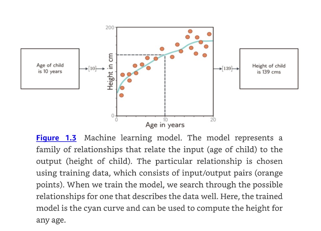
Consider predicting a child’s height from their age. The machine learning model is a mathematical equation describing how average height varies as a function of age — the cyan curve in fig. 3. Run an age of 10 years through it and it returns a height of 139 cm.
Figure 3: Prince (2024), figure 1.3, p. 4.
The subtlety, and it is the single most important idea in the chapter, is that the model is not one curve. The model represents a family of equations — a family of different cyan curves. The particular member of the family is chosen using training data, the input/output pairs shown as orange points.
When we talk about training or fitting a model, we mean that we search through the family of possible equations (possible cyan curves) relating input to output to find the one that describes the training data most accurately.
— Prince, p. 5
Those input/output pairs “take the role of a teacher or supervisor for the training process, and this gives rise to the term supervised learning” (p. 5). The music classifier in fig. 2d needs a large number of audio clips whose genre a human expert has already labeled. Labels are expensive, and that expense is a large part of why unsupervised methods matter.
3.4 Why deep networks
Prince §1.1.4, p. 5.
Deep neural networks are a particularly useful family of equations for two reasons that pull in opposite directions and yet somehow coexist:
They represent an extremely broad family of input/output relationships.
It is nonetheless easy to search that family for the relationship that describes the training data.
Broad families are usually hard to search and easy-to-search families are usually narrow. Getting both is the reason deep learning works at all, and Chapters 6, 7, and 20 return to why.
Deep networks also handle every input difficulty listed above — very large, variable length, internally structured — and can produce single real numbers, multiple numbers, or probabilities over two or more classes. Prince adds that “it is probably hard to imagine equations with these properties, and the reader should endeavor to suspend disbelief for now.” Chapter 3 makes it concrete.
3.5 Structured outputs
Prince §1.1.5, pp. 5–7; figure on p. 6.
Outputs can be as large and structured as inputs.
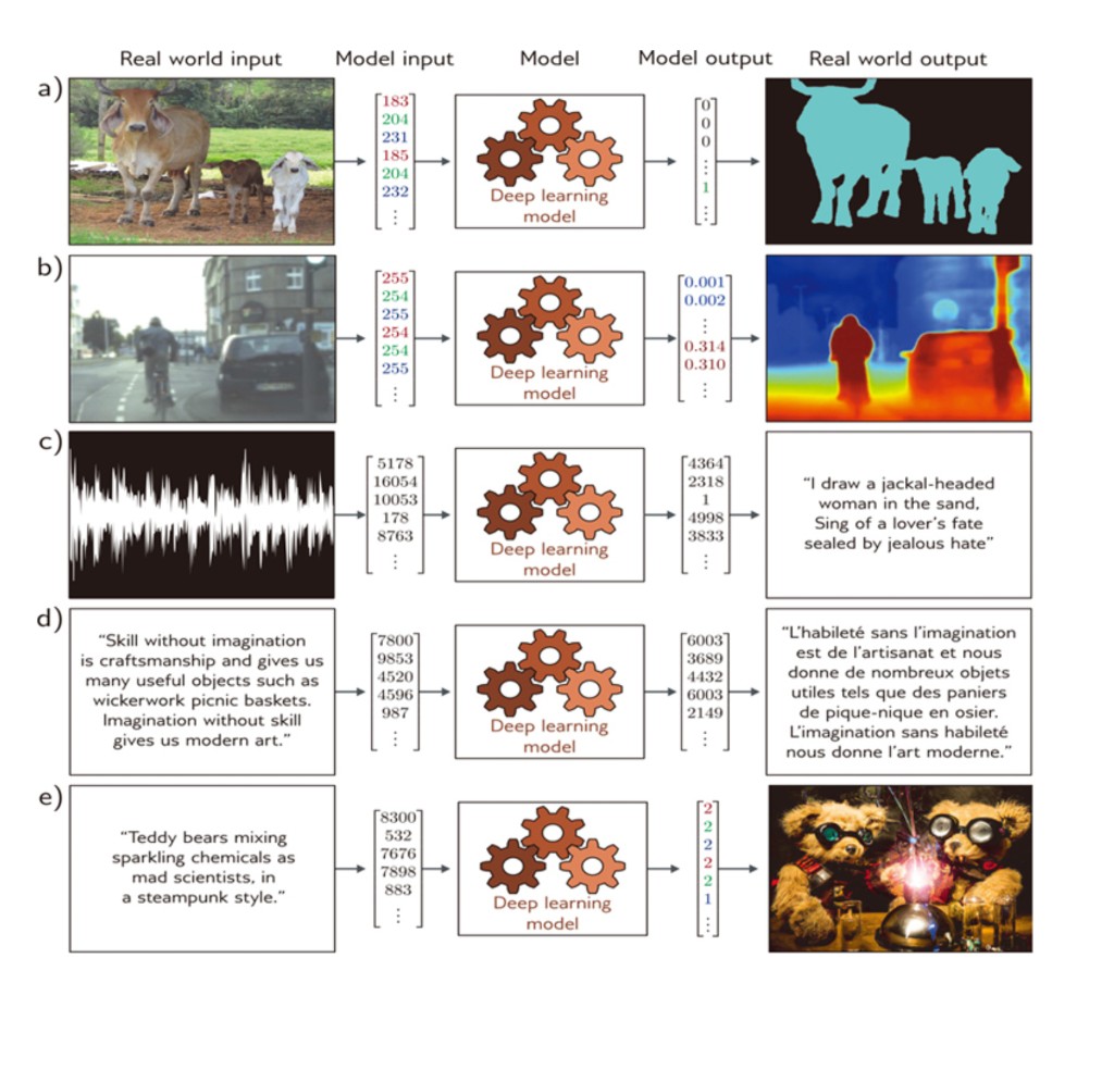
Figure 4: Supervised learning tasks with structured outputs. (a) Semantic segmentation: every pixel gets a binary cow/background label (adapted from Noh et al., 2015). (b) Monocular depth estimation: every pixel gets a depth (adapted from Cordts et al., 2016). (c) Audio transcription. (d) English-to-French translation. (e) Image synthesis from a caption. Prince (2024), figure 1.4, p. 6.
The five panels split into two groups, and the split matters.
In fig. 4a and b the output is high-dimensional and structured, but that structure is closely tied to the input and can therefore be exploited: if a pixel is labeled “cow,” a neighboring pixel with a similar RGB value probably carries the same label. Panel (a) is multivariate binary classification (one label per pixel); panel (b) is multivariate regression (one depth per pixel).
In fig. 4c–e the output structure is not tied so closely to the input, and these are harder for two distinct reasons:
The output may be genuinely ambiguous. There are many valid French translations of an English sentence, and many images compatible with any caption.
The output has its own grammar. Not all strings of words are valid sentences; not all collections of RGB values are plausible images. We have to learn the mapping and respect the grammar of the output space.
The resolution is the hinge of the chapter: that grammar can be learned without output labels, by learning the statistics of a large corpus. Which takes us to unsupervised learning.
4 Unsupervised Learning
Prince §1.2, pp. 7–11.
Constructing a model from input data without corresponding output labels is termed unsupervised learning; the absence of output labels means there can be no “supervision.” Rather than learning a mapping from input to output, the goal is to describe or understand the structure of the data.
— Prince, p. 7
4.1 Generative models
Prince §1.2.1, pp. 7–9; figures on pp. 8–9.
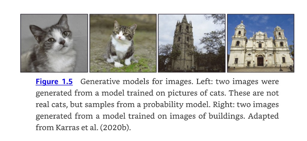
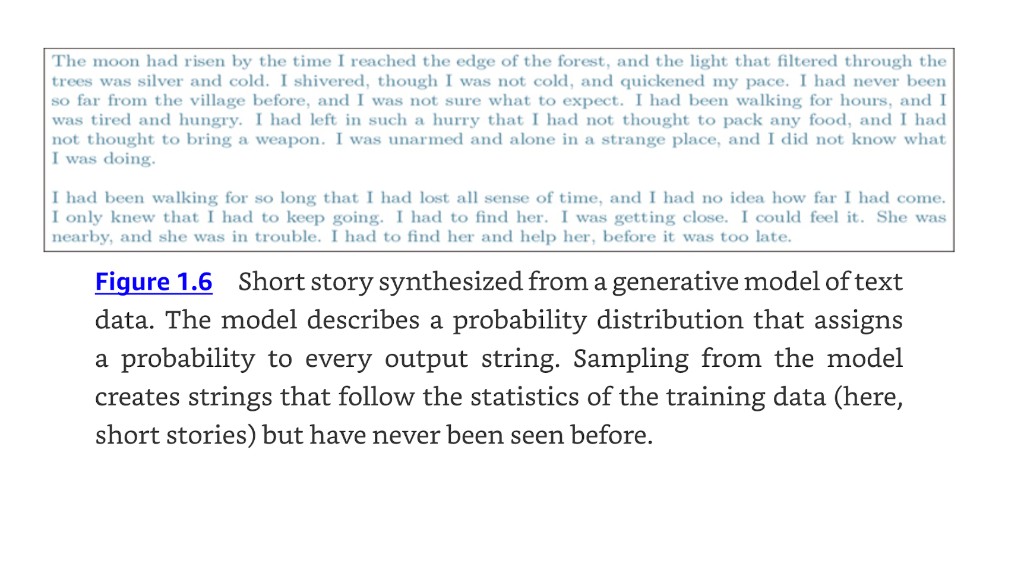
The book focuses on generative unsupervised models: models that learn to synthesize new data examples statistically indistinguishable from the training data. Some describe the probability distribution over the input data explicitly and generate by sampling from it; others merely learn a mechanism for producing new examples without ever writing the distribution down. That distinction separates, for example, variational autoencoders from GANs (Chapter 14).
Figure 5: Prince (2024), figure 1.5, p. 8.
Figure 6: Prince (2024), figure 1.6, p. 8.
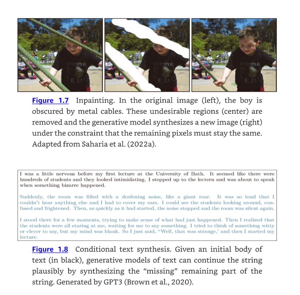
Generative models can also synthesize data under the constraint that some outputs are predetermined, which is called conditional generation. fig. 7 shows the two canonical cases: image inpainting, where the unmasked pixels must stay fixed, and text completion, where the prefix is given.
Figure 7: Prince (2024), figure 1.7 (inpainting) and figure 1.8 (conditional text synthesis), pp. 8–9.
The warning attached to figure 1.8
Prince is explicit about how to read fluent generated text (p. 7): modern generative models of text are so powerful that they “can appear intelligent,” because given a body of text followed by a question the model can fill in the answer by generating the most likely completion of the document. “However, in reality, the model only knows about the statistics of language and does not understand the significance of its answers.”
This is a 2023 sentence about GPT-3, and how much of it still holds is a live argument that we will pick up in Week 12. Read it now as a discipline: an output that reads well is evidence about the model’s language statistics, not about its understanding.
4.2 Latent variables
Prince §1.2.2, pp. 9–11; figures on pp. 9–10.
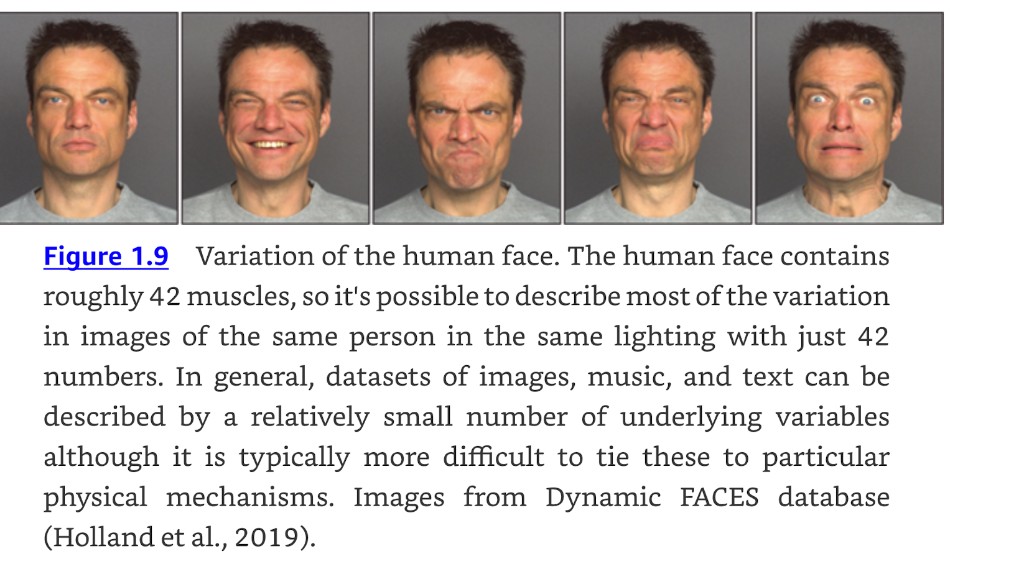
Some generative models exploit an observation about real data: the data are lower dimensional than the raw number of observed variables suggests. The number of valid, meaningful English sentences is vastly smaller than the number of strings you get by drawing words at random. Real-world images are a tiny subset of what you get by drawing random RGB values per pixel, because real images are generated by physical processes.
fig. 8 makes the physical-process argument concrete. The human face has roughly 42 muscles, so most of the variation across images of the same person in the same lighting can be described with about 42 numbers — far fewer than the number of pixels.
Figure 8: Prince (2024), figure 1.9, p. 9.
The following is a cheap way to feel how tiny the subset of “real” images is. Every panel below is a legitimate point in the space of \(32 \times 32\) RGB images. None of them will ever be a photograph.
rng = np.random.default_rng(774)fig, axes = plt.subplots(1, 8, figsize=(11, 1.6))for ax in axes: ax.imshow(rng.integers(0, 256, size=(32, 32, 3), dtype=np.uint8)) ax.set_xticks([]); ax.set_yticks([]); ax.grid(False)plt.tight_layout()plt.show()n_pixels =32*32*3print(f"images in the space : 256^{n_pixels} (about 10^{n_pixels * np.log10(256):.0f})")print(f"atoms in the universe: about 10^80")
Figure 9: Eight uniformly random 32x32 RGB images. The space of such images has \(256^{3072}\) elements; the images a camera can produce occupy a vanishingly small, highly structured region of it. Generative models are in the business of finding that region.
images in the space : 256^3072  (about 10^7398)
atoms in the universe: about 10^80
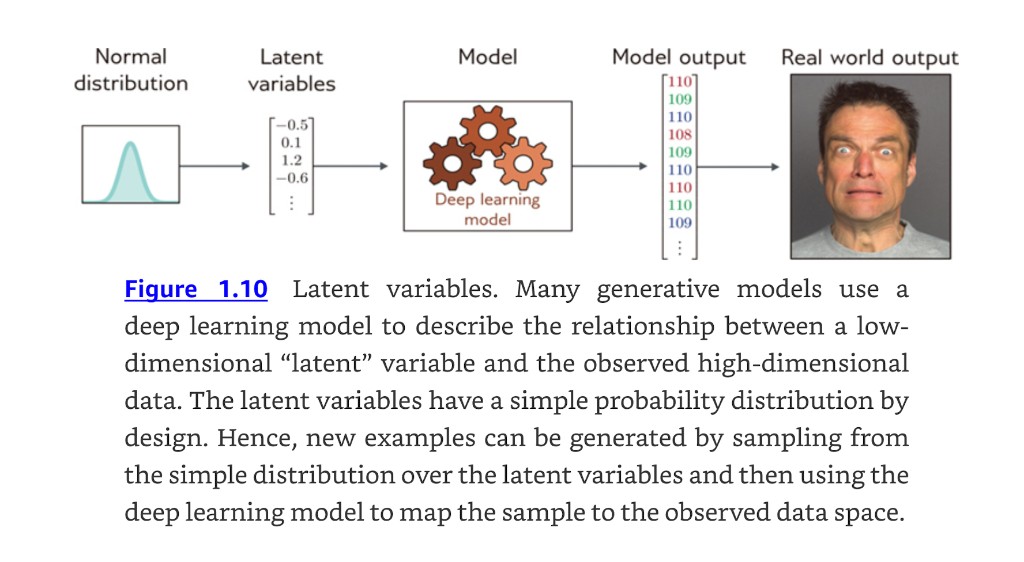
This leads to the central construction: describe each data example using a smaller number of underlying latent variables, and let the deep network describe the mapping from latent variables to data. The latent variables are given a simple probability distribution by design — typically a standard normal. Then generating a new example is two steps: sample a latent vector from the simple distribution, push it through the network.
Figure 10: Prince (2024), figure 1.10, p. 10.
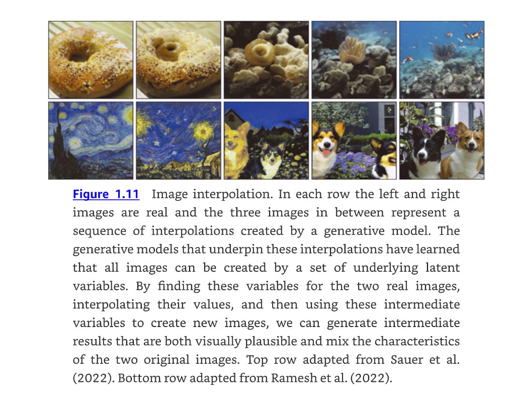
Latents also give us new ways to manipulate real data. Find the latent variables underpinning two real examples, interpolate between them in latent space, and map the intermediate points back to data space. The result is a sequence of plausible examples mixing the characteristics of both, which is not at all what you get from interpolating in pixel space.
Figure 11: Prince (2024), figure 1.11, p. 10.
4.3 Connecting supervised and unsupervised learning
Prince §1.2.3, p. 11; figure on p. 11.
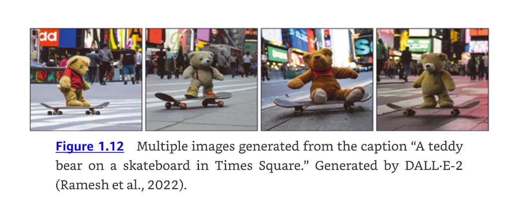
Latent variable models feed back into supervised problems with structured outputs. Rather than mapping a caption directly to an image, learn a relation between the latents that explain the text and the latents that explain the image. Prince lists three advantages (p. 11):
Fewer pairs needed. The inputs and outputs are now low dimensional.
More plausible outputs. Any sensible latent value should decode into something that looks like a real example.
Multiple valid answers. Inject randomness into the latent-to-latent mapping or the latent-to-image mapping, and one caption yields many images — which is the honest response to an ambiguous task.
Figure 12: Prince (2024), figure 1.12, p. 11.
5 Reinforcement Learning
Prince §1.3, pp. 11–13; figure on p. 13.
The third paradigm introduces an agent that lives in a world and can perform certain actions at each time step. Actions change the state of the system, though not necessarily deterministically, and can produce rewards. The goal is to learn to choose actions that lead to high rewards on average.
Two complications define the field.
The temporal credit assignment problem. The reward may arrive long after the action that earned it, so attributing reward to action is not straightforward. Teaching a robot to walk, we might reward it for reaching checkpoints on an obstacle course; reaching a checkpoint takes many joint movements and it is unclear which of them mattered. In chess with a single reward for winning, the problem is extreme: the system must work out which of dozens of moves were instrumental.
The exploration–exploitation trade-off. A robot may discover it can make progress by lying on its side and pushing with one leg. This yields rewards, but far more slowly than balancing and walking. Should it exploit what it knows or explore for something better? Prince frames it as: “should it follow this strategy (exploit what it knows), or should it try different actions to see if it can improve (explore other opportunities)?” (p. 12).
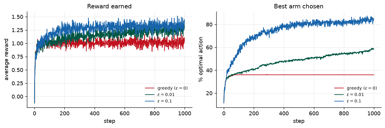
The smallest experiment that shows the trade-off is a multi-armed bandit: \(k\) levers with unknown mean payoffs, and a policy that picks the best-known lever with probability \(1 - \epsilon\) and a random lever otherwise.
Figure 13: Ten-armed bandit averaged over 300 runs. The purely greedy agent (\(\epsilon = 0\)) locks onto whichever arm happened to pay out first and then stops learning, flat at roughly 36% optimal. Both exploring agents beat it. Over this horizon \(\epsilon = 0.1\) is ahead on both measures because it identifies the best arm quickly, but it keeps paying a 10% exploration tax forever. \(\epsilon = 0.01\) is still climbing at step 1,000 and overtakes it eventually, since its tax is only 1%.
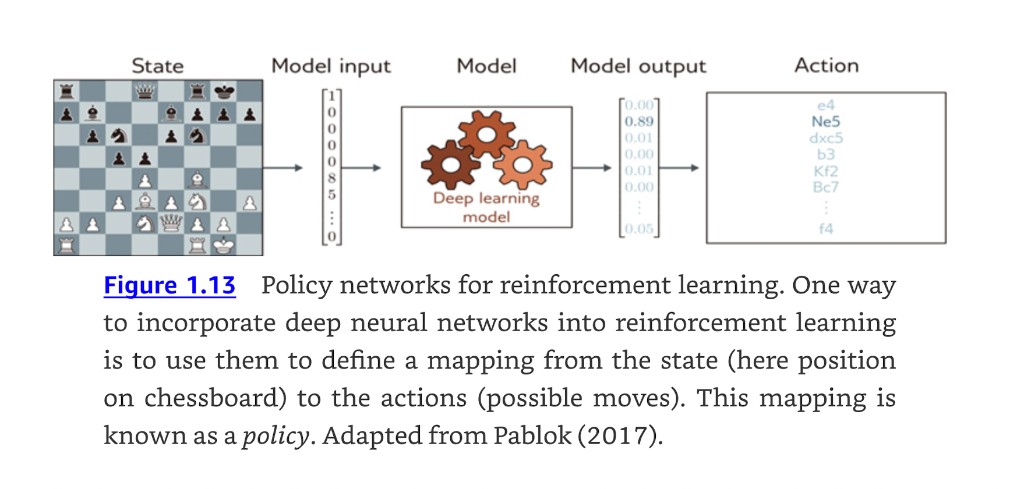
Where does deep learning enter? One route is to use a deep network to map the observed world state to an action. That mapping is called a policy, and the network a policy network. For the robot it maps sensor measurements to joint movements; for chess it maps the board position to a move.
Figure 14: Prince (2024), figure 1.13, p. 13.
Reinforcement learning is Chapter 19 of the textbook and is not a graded topic in this course, but the vocabulary — agent, state, action, reward, policy — recurs whenever we discuss how language models are aligned after pretraining.
6 Ethics
Prince §1.4, pp. 12–14.
Prince argues that it “would be irresponsible to write this book without discussing the ethical implications of artificial intelligence,” and that the technology will change the world at least as much as electricity, the internal combustion engine, the transistor, or the internet. He then notes that “scientists and engineers are often unrealistically optimistic about the outcomes of their work, and the potential for harm is just as great.”
Five concerns, with the citations the book gives:
The five concerns of Prince §1.4, pp. 13–14.
Concern
The argument
Prince’s pointer
Bias and fairness
A system trained on historical salary data reproduces historical bias — it will probably predict that women should be paid less than men. Careless algorithmic decision-making entrenches or aggravates existing bias.
Binns (2018)
Explainability
Systems with billions of parameters make decisions we cannot account for by inspection. Local explanations — why this decision — are moderately successful; whether fully transparent complex systems are possible at all is unknown.
Grennan et al. (2022)
Weaponizing AI
Every significant technology has been applied to war, directly or indirectly. AI is arguably the most powerful ever built and is already being deployed militarily.
Heikkilä (2022)
Concentrating power
The world’s most powerful companies are not investing out of benevolence. Deep learning concentrates power in the few organizations that control it, and automation disproportionately affects lower-paid workers.
David (2015)
Existential risk
The major existential risks all stem from technology. We should be cautious about building systems more capable and extensible than ourselves — in the best case that puts vast power in the owners’ hands, in the worst we cannot control or even understand it.
Tegmark (2018)
The list is not exhaustive. Prince also names surveillance, disinformation, privacy violations, fraud, financial market manipulation, and the climate cost of training. His historical argument is the one worth sitting with: the online community of the eighties and early nineties could hardly have predicted spam, fake news, online harassment, doxxing, or radicalization. Harms from new technology tend to arrive in forms nobody modeled.
What he asks of us specifically
Prince addresses instructors and students directly (p. 14): “If you are a professor teaching from this book, you are encouraged to raise these issues with your students. If you are a student taking a course where this is not done, then lobby your professor to make this happen.”
Consider this section that request being honored, and the invitation standing all semester. The online course at ethics-of-ai.mooc.fi is the introductory resource the book recommends.
7 How the Book and the Course Are Organized
Prince §1.5–§1.7, pp. 15–16.
The book’s structure follows the structure of Chapter 1, and our schedule follows the book.
Book structure from §1.5, p. 15, mapped onto the course schedule.
Chapters
Content
Our weeks
2–9
The supervised learning pipeline: shallow and deep networks, how to train them, how to measure and improve performance
1–9
10–13
Architectural variations used across all three paradigms: convolutional networks, residual connections, transformers
Deep reinforcement learning (necessarily superficial, by the author’s own description)
not covered
20
Open questions: why are deep networks easy to train, why do they generalize, why so many parameters, do they need to be deep — plus double descent, grokking, and lottery tickets
woven through
21
Ethics and deep learning
woven through
On how to read it (§1.7, p. 16): each chapter has a main body, a notes section, and problems. The main body is self-contained. The notes give historical development and pointers for further reading and are less self-contained. Problems are referenced in the margin at the point they should be attempted, and starred problems have answers on the UDL website. Prince quotes Pólya — “Mathematics, you see, is not a spectator sport” — and recommends attempting problems as you go. Notebook 1.1 on background mathematics is the one to work through this week if you are rusty.
Chapter 1 itself has no problems; the exercises below are ours plus the Chapter 2 problem set.
8 Supervised Learning, Formalized
Prince §2.1, pp. 17–18.
Session 2 turns the informal account of §1.1 into notation we will use for the rest of the semester.
We want a model that takes an input \(\mathbf{x}\) and produces a prediction \(\mathbf{y}\):
\[
\mathbf{y} = \mathbf{f}[\mathbf{x}].
\tag{1}\]
Computing \(\mathbf{y}\) from \(\mathbf{x}\) is called inference.
The model is an equation of fixed form, so it represents a family of relations rather than one. Which member of the family we get is determined by the parameters\(\boldsymbol{\phi}\), so we should really write:
Training means finding parameters that make sensible predictions. We use a training dataset of \(I\) input/output pairs \(\{\mathbf{x}_i, \mathbf{y}_i\}\) and quantify the mismatch with a scalar loss\(L[\boldsymbol{\phi}]\). Training is then a minimization:
Afterwards we run the model on separate test data to see how well it generalizes to examples it did not see during training.
Notation
Prince uses square brackets \(f[\cdot]\) for function application, reserving parentheses for grouping. Vectors are bold lowercase, matrices bold uppercase. The loss also depends on the training data, so strictly it is \(L[\{\mathbf{x}_i, \mathbf{y}_i\}, \boldsymbol{\phi}]\), but that is cumbersome and the data are dropped by convention (p. 18, footnote 1). Appendix A collects the full notation.
9 Linear Regression: The Whole Recipe in Miniature
Prince §2.2, pp. 18–22; figures on pp. 19–23.
Everything above appears in the simplest possible model, which is worth walking through completely because every later chapter is a variation on it.
Two parameters, \(\boldsymbol{\phi} = [\phi_0, \phi_1]^T\): a \(y\)-intercept and a slope. eq. 4 defines a family of input/output relations — all possible lines — and the parameters pick the member.
9.2 The loss
Prince §2.2.2, pp. 19–21.
Mismatch is the deviation between the prediction \(f[x_i, \boldsymbol{\phi}]\) and the ground truth \(y_i\). Sum the squares over all \(I\) pairs:
This is the least-squares loss. Squaring makes the direction of the deviation irrelevant — a point above the line is as wrong as a point below it — and there are theoretical reasons for the choice that Chapter 5 supplies. Training is eq. 3 applied to eq. 5.
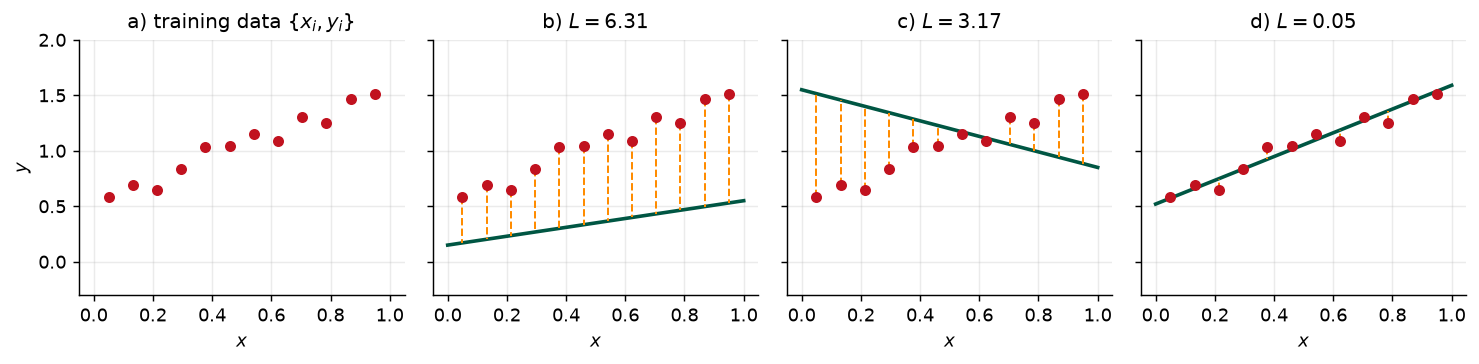
I =12x = np.linspace(0.05, 0.95, I)y =0.5+1.1* x + np.random.normal(0, 0.08, I)def loss(phi0, phi1):return np.sum((phi0 + phi1 * x - y) **2)candidates = [(0.15, 0.40), (1.55, -0.70), (0.52, 1.07)]grid = np.linspace(0, 1, 100)fig, axes = plt.subplots(1, 4, figsize=(11.5, 2.9), sharex=True, sharey=True)axes[0].scatter(x, y, s=26, color=ACCENT, zorder=3)axes[0].set_title("a) training data $\\{x_i, y_i\\}$")axes[0].set_ylabel("$y$")for ax, letter, (p0, p1) inzip(axes[1:], "bcd", candidates): ax.scatter(x, y, s=26, color=ACCENT, zorder=3) ax.plot(grid, p0 + p1 * grid, color=NDSU_GREEN, lw=2) ax.vlines(x, y, p0 + p1 * x, color="darkorange", ls="--", lw=1.1) ax.set_title(f"{letter}) $L = {loss(p0, p1):.2f}$")for ax in axes: ax.set_xlabel("$x$") ax.set_ylim(-0.3, 2.0)plt.tight_layout()plt.show()
Figure 15: Our version of Prince figures 2.2a–d, p. 20. Panel (a) is the training data, \(I = 12\) input/output pairs. Panels (b)–(d) show three choices of \(\boldsymbol{\phi}\); orange dashed lines are the deviations whose squares are summed in eq. 5. The losses span more than two orders of magnitude, and the ordering matches the visual quality of the fits.
With only two parameters we can evaluate the loss for every combination and look at the whole thing as a surface.
9.3 Training
Prince §2.2.3, p. 22; figure on p. 23.
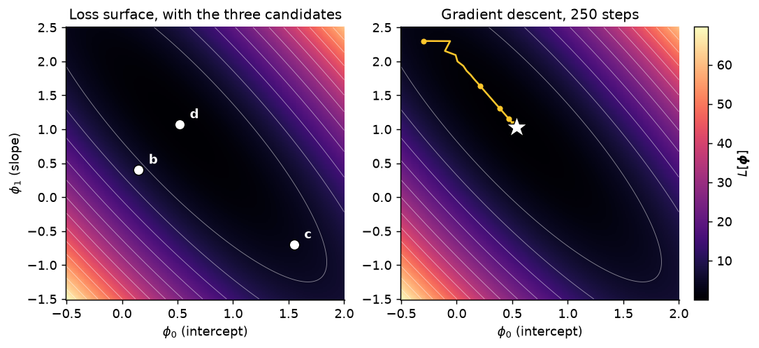
Finding the parameters that minimize the loss is called model fitting, training, or learning. The basic method: initialize randomly, then improve by “walking downhill” on the loss surface. Measure the gradient at the current position, step in the most steeply downhill direction, repeat until the gradient is flat.
p0_grid, p1_grid = np.meshgrid(np.linspace(-0.5, 2.0, 220), np.linspace(-1.5, 2.5, 220))L = ((p0_grid[..., None] + p1_grid[..., None] * x - y) **2).sum(axis=-1)def grad(phi0, phi1): resid = phi0 + phi1 * x - yreturn2* resid.sum(), 2* (resid * x).sum()path = [(-0.3, 2.3)]lr, n_steps =0.05, 250for _ inrange(n_steps): g0, g1 = grad(*path[-1]) path.append((path[-1][0] - lr * g0, path[-1][1] - lr * g1))path = np.array(path)# Least squares has a closed form, so we know the exact answer to compare against.A = np.column_stack([np.ones(I), x])phi_star = np.linalg.lstsq(A, y, rcond=None)[0]fig, axes = plt.subplots(1, 2, figsize=(10.5, 3.9))for ax in axes: im = ax.pcolormesh(p0_grid, p1_grid, L, cmap="magma", shading="auto") ax.contour(p0_grid, p1_grid, L, levels=14, colors="white", linewidths=0.5, alpha=0.5) ax.set_xlabel("$\\phi_0$ (intercept)") ax.grid(False)axes[0].set_ylabel("$\\phi_1$ (slope)")for (p0, p1), letter inzip(candidates, "bcd"): axes[0].plot(p0, p1, "o", color="white", ms=8, mec="k", mew=0.8, zorder=4) axes[0].annotate(letter, (p0, p1), textcoords="offset points", xytext=(8, 5), color="white", fontweight="bold")axes[0].set_title("Loss surface, with the three candidates")axes[1].plot(path[:, 0], path[:, 1], color=NDSU_GOLD, lw=1.4, zorder=4)axes[1].plot(path[::10, 0], path[::10, 1], "o", color=NDSU_GOLD, ms=3.5, zorder=4)axes[1].plot(*phi_star, "*", color="white", ms=18, mec="k", mew=0.8, zorder=5)axes[1].set_title(f"Gradient descent, {n_steps} steps")fig.colorbar(im, ax=axes, label="$L[\\boldsymbol{\\phi}]$", pad=0.02)plt.show()print(f"gradient descent, {n_steps} steps : phi0 = {path[-1, 0]:.4f}, phi1 = {path[-1, 1]:.4f}")print(f"closed-form least squares : phi0 = {phi_star[0]:.4f}, phi1 = {phi_star[1]:.4f}")
Figure 16: Our version of Prince figures 2.3 and 2.4, pp. 21 and 23. Left: the loss eq. 5 as a heatmap over the two parameters, with the three candidate lines from fig. 15 marked. Right: gradient descent from a random start, stepping downhill perpendicular to the contours toward the minimum (white star); markers are every tenth step. The valley is long and narrow, so most of the 250 steps are spent creeping along its floor rather than descending into it — an early glimpse of the conditioning problems Chapter 6 confronts.
The iterative approach is unnecessary here — linear regression has a closed-form solution, which is why the two lines of output agree. We use gradient descent anyway because it generalizes to models where no closed form exists and where there are far too many parameters to evaluate the loss on a grid. Chapter 6 makes this precise.
Here is the same fit in PyTorch, which is how every model in this course will actually be written:
Training loss tells us nothing on its own. We compute the loss on a separate set of test data to see how the model performs in the real world. How well accuracy generalizes depends on two things:
How representative and complete the training data is.
How expressive the model is. A line may be unable to capture the true relationship, which is underfitting. A very expressive model may instead describe statistical peculiarities of the training data that are atypical, producing unusual predictions, which is overfitting.
Chapter 8 measures this properly and Chapter 9 fights it with regularization.
10 Summary
Prince §2.3, p. 22.
Machine learning fits mathematical models to observed data and splits into supervised, unsupervised, and reinforcement learning; deep networks are the leading method in all three.
A supervised model is a function \(\mathbf{y} = \mathbf{f}[\mathbf{x},
\boldsymbol{\phi}]\) relating inputs to outputs, where \(\boldsymbol{\phi}\) selects one relationship out of a family. To train it we define a loss \(L[\boldsymbol{\phi}]\) over a training set \(\{\mathbf{x}_i, \mathbf{y}_i\}\) quantifying the mismatch between predictions and observed outputs, and search for the parameters that minimize it. We then evaluate on separate test data.
Unsupervised learning drops the output labels and asks instead for the structure of the data. Generative models synthesize new examples; the ones built on latent variables assume the data lie near a low-dimensional manifold and use a deep network to map simple latents to complex data.
Reinforcement learning adds an agent, actions, and delayed rewards, and inherits two problems the other paradigms do not have: temporal credit assignment and the exploration–exploitation trade-off.
Next: Chapter 3 replaces the straight line of eq. 4 with a shallow neural network, which is only slightly more complicated but describes a vastly larger family of relationships.
11 Exercises
Chapter 1 of Prince has no problem set. Problems 1–5 below are ours; problems 6–8 are Prince problems 2.1–2.3 (p. 24). Starred UDL problems have answers on the UDL website.
1. For each of the following, say whether it is supervised, unsupervised, or reinforcement learning, and if supervised, which of the four output types in fig. 2 it uses. (a) Predicting remaining useful life of a bearing from vibration spectra. (b) Clustering warehouse SKUs by demand pattern. (c) Choosing which machine to run next on a shop floor to minimize makespan. (d) Flagging a weld as pass/fail from an X-ray image. (e) Generating a synthetic defect image to augment a small training set.
2. Prince says tabular data has “no internal structure; if we change the order of the inputs and build a new model, then we expect the model prediction to remain the same” (p. 2). Explain why the same statement is false for the image in fig. 2e, and name the property of images that a convolutional network exploits instead.
3.fig. 4 splits into two groups: (a)–(b), where output structure is tied closely to the input, and (c)–(e), where it is not. Place these three tasks in the correct group and justify each: optical character recognition on a scanned page; predicting a protein’s 3D structure from its amino acid sequence; generating a product description from a photograph.
4. The face in fig. 8 is argued to need roughly 42 numbers because the face has roughly 42 muscles. Give the analogous argument for a dataset of photographs of a single manufactured part on a fixed inspection rig, and estimate the latent dimension. What breaks your estimate?
5. Pick one of the five concerns in §1.4 and one deep learning application in your own field. Write a paragraph identifying a concrete way that concern could materialize, and one design or process decision that would reduce it. Be specific enough that someone could disagree with you.
6. (UDL 2.1) To walk downhill on the loss function eq. 5 we need its gradient with respect to \(\phi_0\) and \(\phi_1\). Derive expressions for \(\partial L / \partial \phi_0\) and \(\partial L / \partial \phi_1\), and check them against the grad function in the code above.
7. (UDL 2.2) Show that the minimum of the loss function can be found in closed form by setting the derivatives from the previous problem to zero and solving. Note where this argument fails for more complex models — which is why we use iterative methods.
8. (UDL 2.3*) Reformulate linear regression as a generative model, so \(x = g[y, \boldsymbol{\phi}] = \phi_0 + \phi_1 y\). What is the new loss function? Find \(y = g^{-1}[x, \boldsymbol{\phi}]\), which is what we would use for inference. Will this model make the same predictions as the discriminative version on a given dataset? Fit a line to three points both ways in code and compare.
9. Computational. Re-run the bandit experiment in fig. 13 with \(\epsilon \in \{0, 0.01, 0.1, 0.5\}\) for 20,000 steps. Which \(\epsilon\) leads at step 100, at step 1,000, and at the end? Find roughly where \(\epsilon = 0.01\) overtakes \(\epsilon = 0.1\), and explain both the crossover and why \(\epsilon = 0.5\) never competes, in terms of the exploration–exploitation trade-off.
10. Computational. Add a single outlier at \((0.5, 5.0)\) to the linear regression data and re-fit. How much do \(\phi_0\) and \(\phi_1\) move? Explain using the squaring in eq. 5, then try minimizing the sum of absolute deviations instead and compare.
12 Textbook Reference Map
Every part of this page, mapped to Prince, Understanding Deep Learning (MIT Press, 2024) (Prince 2024). Page numbers are those of the printed book.
Equations on this page correspond to Prince as follows: eq. 1 is his (2.1), eq. 2 is (2.2), eq. 3 is (2.3), eq. 4 is (2.4), and eq. 5 is (2.5). His (2.6) is eq. 3 applied to eq. 5.
Figure credits
Figures 1.1–1.13 are reproduced unaltered from Prince, Understanding Deep Learning (MIT Press, 2024), which is distributed under a Creative Commons CC-BY-NC-ND license, and are used here for non-commercial classroom instruction. Original sources credited within the figures: Noh et al. (2015); Cordts et al. (2016); Karras et al. (2020b); Saharia et al. (2022a); Brown et al. (2020); Holland et al. (2019), Dynamic FACES database; Sauer et al. (2022); Ramesh et al. (2022); Pablok (2017). All other figures on this page are generated by the code shown.
13 Further Reading
The book’s own recommendations, from §1.6 (p. 15):
Prince, Understanding Deep Learning, Chapters 1–2 (Prince 2024) — the assigned reading. Notebook 1.1 covers the background mathematics.
Goodfellow, Bengio & Courville, Deep Learning(Goodfellow, Bengio, and Courville 2016) — the book Prince describes as the one he intends this to succeed. Excellent, but predates the recent advances.
Murphy, Probabilistic Machine Learning (2022, 2023) — the most up-to-date encyclopedic treatment of machine learning generally.
Bishop, Pattern Recognition and Machine Learning (2006) — older, still excellent and relevant.
Prince, Computer Vision: Models, Learning, and Inference (2012) — same notation as the textbook; thorough introduction to probability and latent variable models, available online.
Deisenroth, Faisal & Ong, Mathematics for Machine Learning (2020) — the background mathematics reference if Appendix B moves too fast.
Zhang et al., Dive into Deep Learning (2023) — a coding-first alternative presentation.
Sutton & Barto, Reinforcement Learning: An Introduction (2018) — the definitive reinforcement learning text, if fig. 13 interested you.