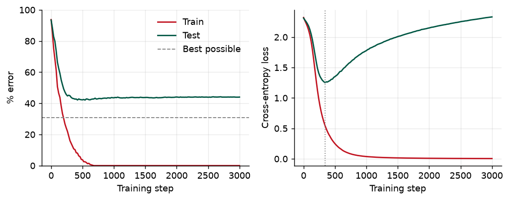
best achievable test error (nearest class mean): 30.7%
lowest test loss 1.251 at step 340, where test error is 43.2%
after 3,000 steps: train error 0.0%, train loss 0.0044; test error 44.0%, test loss 2.331Week 8 · Sessions 15–16 · October 13 & 15, 2026
Every section below opens with the section number and page range it covers in Prince, Understanding Deep Learning (MIT Press, 2024). Page numbers are those of the printed book. Figures taken from the textbook are captioned with their original figure number and page; figures generated by the code behind this page are ours. A complete cross-reference table appears in Section 12.
By the end of this week you should be able to:
This page shows the figures and results; the Python behind them is not printed here. All of it — every cell, in the order the note uses it — is in a notebook you can open in the browser with nothing to install:
Colab gives you a Python environment with NumPy, matplotlib, and PyTorch already installed. In Colab, run a cell with Shift+Enter. If you prefer to work locally, pip install -r requirements.txt from the course repository gives you the same environment.
Prince, Chapter 8 opening, p. 118.
Weeks 4–7 gave us everything needed to train a network: a model, a loss, an optimizer, an initialization, and backpropagation to compute the gradients. Run that machinery on a network with enough hidden units and it will often classify the training data perfectly. That tells us almost nothing about what we actually care about, which is how the network does on examples it has never seen — how well it generalizes.
This chapter makes that question precise. Prince shows that test error has three distinct causes, and that how much each contributes depends on three things: how much inherent uncertainty the task has, how much training data we have, and which model we chose. The last of these raises a practical problem that occupies the end of the chapter: how to choose the hyperparameters — the number of layers and hidden units, the learning rate, the batch size, and so on — that training itself does not choose.
Prince §8.1, pp. 118–120; figures on p. 119.
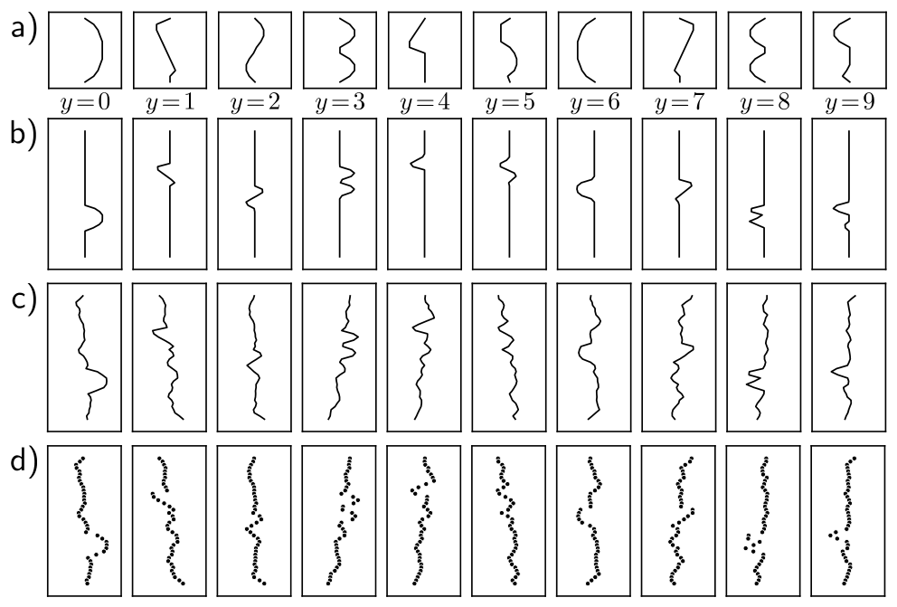
Prince’s running example is MNIST-1D (Greydanus 2020), a deliberately small stand-in for the MNIST handwritten digits. There are ten classes \(y \in \{0, 1, \ldots, 9\}\), one per digit. Each class has a one-dimensional template, and each data example \(\mathbf{x}\) is made by randomly transforming a template, adding noise, and sampling the result at \(D_i = 40\) positions (fig. 1). The training set has \(I = 4{,}000\) examples, about 400 per class.
The network has 40 inputs, two hidden layers of 100 units, and 10 outputs that pass through a softmax (Week 5). It is trained with SGD — batch size 100, learning rate 0.1 — for 6,000 steps (150 epochs) on the multiclass cross-entropy loss. The training error falls steadily and reaches zero after about 4,000 steps; the training loss heads toward zero too (fig. 2).
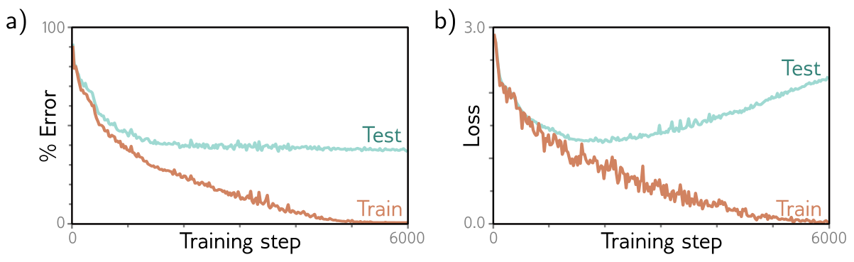
Perfect training performance does not mean a perfect classifier: the network may simply have memorized the training set. To find out, we need a separate test set, generated by the same process but never used in training. Prince draws 1,000 more examples. The test error falls during training, but only to about 40% — far better than the 90% of random guessing, far worse than the 0% on the training set. The model has not generalized well.
The test loss tells a stranger story. It falls for the first 1,500 steps or so and then rises, even though the test error has stopped changing. The network is making the same mistakes with ever greater confidence. To push the probability of every training label toward one, training drives the pre-softmax activations to more and more extreme values (recall Prince’s figure 5.10 from Week 5). On a test example the network gets wrong, that same extremity pushes the probability of the correct class toward zero, and the negative log-likelihood of that example grows without bound.
We can reproduce the whole effect in a couple of seconds with a synthetic problem of the same shape: ten classes, 40-dimensional inputs, and the same network and optimizer, but only 400 training examples. Each class is a Gaussian blob around its own mean. Because we generated the data, we also know the best error any classifier could achieve: assigning each test point to the nearest class mean is optimal here, and it still errs about 31% of the time, because the blobs overlap.
best achievable test error (nearest class mean): 30.7%
lowest test loss 1.251 at step 340, where test error is 43.2%
after 3,000 steps: train error 0.0%, train loss 0.0044; test error 44.0%, test loss 2.331Two lessons carry through the rest of the chapter. First, the training numbers are not evidence of anything; only held-out data can tell us how the model will do. Second, error and loss can disagree. The classification error is what we usually report, but the loss is what the network optimizes, and a rising test loss with a flat test error is the signature of a model growing overconfident.
Prince §8.2, pp. 120–122; figures on pp. 120–122.
To see why a model fails to generalize, Prince switches to a problem where we know the ground truth exactly: one-dimensional least squares regression. Inputs are drawn from \([0, 1]\), outputs are a fixed quasi-sinusoidal function plus Gaussian noise of fixed variance, and training and test data come from the same process. To spread \(I\) training inputs evenly, \([0, 1]\) is cut into \(I\) equal segments and one \(x_i\) is drawn uniformly from each (fig. 4).
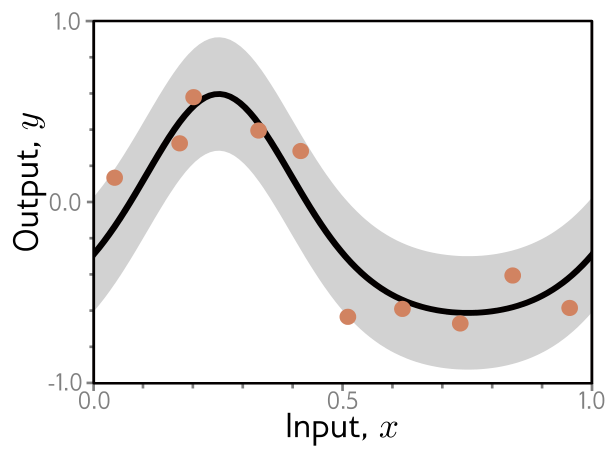
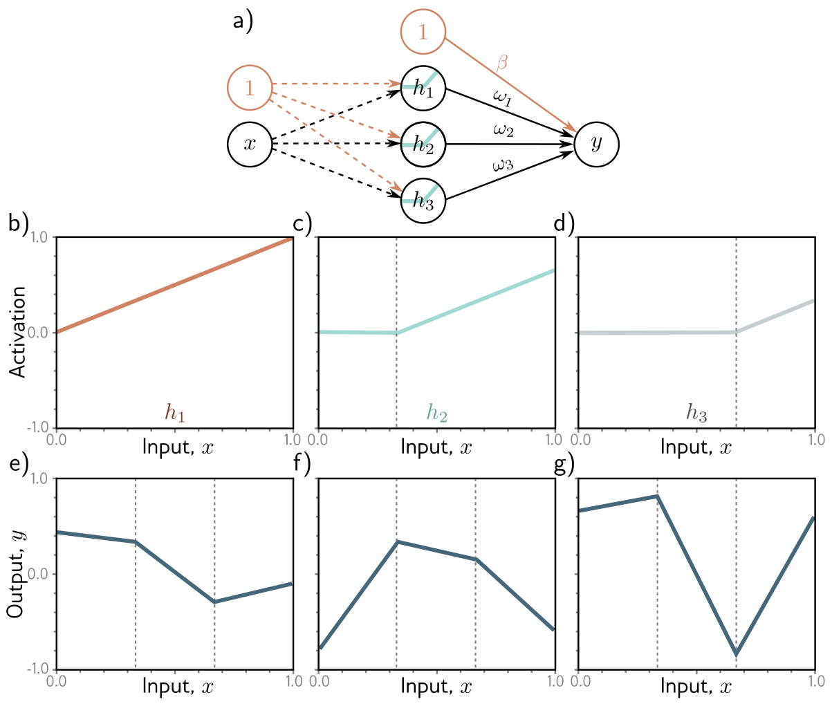
The model is a simplified shallow network (fig. 5). With \(D\) hidden units, the first-layer weights and biases are fixed so that each hidden unit is a ReLU of slope one whose joint sits at \(0, 1/D, 2/D, \ldots, (D-1)/D\). Only the output layer, \(\boldsymbol{\phi} = \{\beta, \omega_1, \ldots, \omega_D\}\), is learned. The model can represent any piecewise linear function on \([0, 1]\) with \(D\) equal-width linear regions. Because it is linear in \(\boldsymbol{\phi}\), its least squares fit has a closed form (problem 8.3), so we are guaranteed the global minimum of the training loss — any error we see is the model’s fault or the data’s, never the optimizer’s.
Prince §8.2.1, pp. 122–123; figure on p. 122.
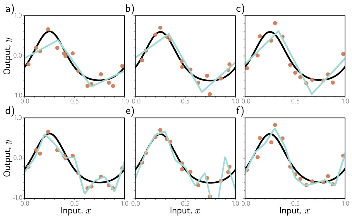
There are three possible sources of test error (fig. 6).
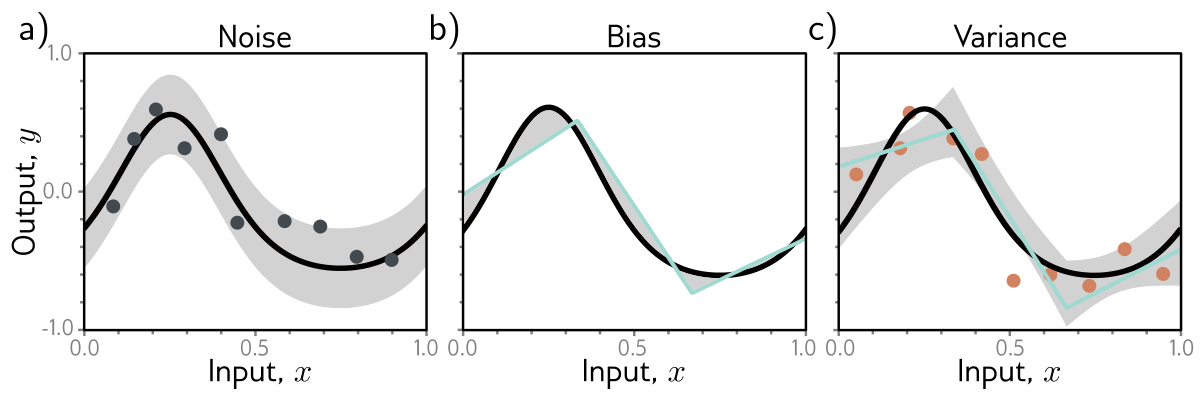
Noise. The data-generating process itself is random, so a single input \(x\) has many valid outputs \(y\). Even a model that reproduced the true underlying function exactly would still miss the test points by the noise (panel a). Noise is insurmountable on test data. It does not, however, limit training performance: we will almost never see the same \(x\) twice, so a flexible enough model can still pass through every training point. Noise arises from genuine randomness, from mislabeled data, or from explanatory variables we did not observe — in a plant, an unmeasured ambient temperature or tool-wear state looks exactly like noise to a model that cannot see it. Occasionally there is no noise (a network approximating an expensive deterministic simulation, for instance), but usually noise sets a floor on test performance. In fig. 3 the floor was the 31% error of the best possible classifier.
Bias. The model may not be flexible enough to represent the true function, even with its parameters set optimally. The three-region model cannot trace the quasi-sinusoid however we choose \(\boldsymbol{\phi}\) (panel b). This systematic shortfall is the bias.
Variance. We have only a limited, noisy training set, and the fit cannot tell which wiggles in it belong to the underlying function and which are noise. So we do not recover the best possible function of panel b; we recover one that reflects the quirks of our particular sample, and a different sample would give a different fit (panel c). This extra variability is the variance. With a stochastic optimizer there is more: two training runs on the same data need not converge to the same solution.
Prince §8.2.2, pp. 123–124.
We now make the three terms exact for one-dimensional regression with additive noise of variance \(\sigma^2\). Because the same \(x\) can produce different \(y\), each input has a distribution \(Pr(y|x)\) with mean
\[ \mu[x] = \mathbb{E}_y\big[y[x]\big] = \int y[x]\, Pr(y|x)\, dy, \tag{1}\]
and the noise is \(\sigma^2 = \mathbb{E}_y\big[(\mu[x] - y[x])^2\big]\). The notation \(y[x]\) is a reminder that we are looking at the output at one fixed input position \(x\).
\(\mathbb{E}_y[\bullet]\) averages over the noise in a test output; \(\mathbb{E}_{\mathcal{D}}[\bullet]\), below, averages over random training sets \(\mathcal{D} = \{x_i, y_i\}\). The function \(\mu[x]\) is the true mean output and \(f_\mu[x]\) is the average fitted model. Neither can be computed in practice: one needs the true process, the other infinitely many training sets. They exist to make the decomposition exact. Appendix C.2 reviews the rules for expectations used below.
Step 1: split off the noise. Take the least squares loss at position \(x\), then add and subtract \(\mu[x]\) inside the square and expand:
\[ \begin{aligned} L[x] &= \big(\mathrm{f}[x, \boldsymbol{\phi}] - y[x]\big)^2 \\ &= \Big(\big(\mathrm{f}[x, \boldsymbol{\phi}] - \mu[x]\big) + \big(\mu[x] - y[x]\big)\Big)^2 \\ &= \big(\mathrm{f}[x, \boldsymbol{\phi}] - \mu[x]\big)^2 + 2\big(\mathrm{f}[x, \boldsymbol{\phi}] - \mu[x]\big)\big(\mu[x] - y[x]\big) + \big(\mu[x] - y[x]\big)^2. \end{aligned} \tag{2}\]
The loss depends on which \(y[x]\) we happen to observe, so take its expectation. The model term does not depend on \(y\), so the expectation passes it untouched; the cross term vanishes because \(\mathbb{E}_y[y[x]] = \mu[x]\) by definition; and the last term is \(\sigma^2\) by definition:
\[ \begin{aligned} \mathbb{E}_y\big[L[x]\big] &= \big(\mathrm{f}[x, \boldsymbol{\phi}] - \mu[x]\big)^2 + 2\big(\mathrm{f}[x, \boldsymbol{\phi}] - \mu[x]\big)\big(\mu[x] - \mathbb{E}_y[y[x]]\big) + \mathbb{E}_y\big[(\mu[x] - y[x])^2\big] \\ &= \big(\mathrm{f}[x, \boldsymbol{\phi}] - \mu[x]\big)^2 + 2\big(\mathrm{f}[x, \boldsymbol{\phi}] - \mu[x]\big) \cdot 0 + \sigma^2 \\ &= \big(\mathrm{f}[x, \boldsymbol{\phi}] - \mu[x]\big)^2 + \sigma^2. \end{aligned} \tag{3}\]
So the expected loss is the squared distance between the model and the true mean, plus the noise.
Step 2: split the model term into bias and variance. The parameters were learned from a training set \(\mathcal{D}\), so properly we should write \(\boldsymbol{\phi}[\mathcal{D}]\). The training set is a random sample; a different sample gives different parameters. The model’s average output over all possible training sets is
\[ f_\mu[x] = \mathbb{E}_{\mathcal{D}}\Big[\mathrm{f}\big[x, \boldsymbol{\phi}[\mathcal{D}]\big]\Big]. \tag{4}\]
Repeat the trick on the first term of eq. 3, adding and subtracting \(f_\mu[x]\) this time:
\[ \begin{aligned} \big(\mathrm{f}[x, \boldsymbol{\phi}[\mathcal{D}]] - \mu[x]\big)^2 &= \Big(\big(\mathrm{f}[x, \boldsymbol{\phi}[\mathcal{D}]] - f_\mu[x]\big) + \big(f_\mu[x] - \mu[x]\big)\Big)^2 \\ &= \big(\mathrm{f}[x, \boldsymbol{\phi}[\mathcal{D}]] - f_\mu[x]\big)^2 + 2\big(\mathrm{f}[x, \boldsymbol{\phi}[\mathcal{D}]] - f_\mu[x]\big)\big(f_\mu[x] - \mu[x]\big) + \big(f_\mu[x] - \mu[x]\big)^2. \end{aligned} \tag{5}\]
Taking the expectation over \(\mathcal{D}\) kills the cross term for the same reason as before, since \(\mathbb{E}_{\mathcal{D}}\big[\mathrm{f}[x, \boldsymbol{\phi}[\mathcal{D}]]\big] = f_\mu[x]\):
\[ \mathbb{E}_{\mathcal{D}}\Big[\big(\mathrm{f}[x, \boldsymbol{\phi}[\mathcal{D}]] - \mu[x]\big)^2\Big] = \mathbb{E}_{\mathcal{D}}\Big[\big(\mathrm{f}[x, \boldsymbol{\phi}[\mathcal{D}]] - f_\mu[x]\big)^2\Big] + \big(f_\mu[x] - \mu[x]\big)^2. \tag{6}\]
Step 3: put it together. Substituting eq. 6 into eq. 3:
\[ \mathbb{E}_{\mathcal{D}}\Big[\mathbb{E}_y\big[L[x]\big]\Big] = \underbrace{\mathbb{E}_{\mathcal{D}}\Big[\big(\mathrm{f}[x, \boldsymbol{\phi}[\mathcal{D}]] - f_\mu[x]\big)^2\Big]}_{\text{variance}} + \underbrace{\big(f_\mu[x] - \mu[x]\big)^2}_{\text{bias}} + \underbrace{\sigma^2}_{\text{noise}}. \tag{7}\]
The variance is how much the fitted model moves around with the training set we happen to draw. The bias is how far the average fitted model sits from the true mean. The noise is the uncertainty in the true mapping from input to output.
Two remarks. First, the “bias” term is a squared bias; Prince follows common usage and calls it the bias. Second, the three terms are present for any task, but they add this cleanly only for least squares regression. For other losses their interaction is more complicated: in classification, more variance can even help, if it pushes some predictions in a region where the model is biased toward the wrong class back over the decision threshold (chapter notes, pp. 133–134).
The decomposition is exact, so we can check it. The cell below builds Prince’s simplified model in a few lines — its features are a column of ones plus one shifted ReLU per hidden unit, and np.linalg.lstsq gives the global least squares fit. Our true function is our own quasi-sinusoid with \(\sigma = 0.15\). We then estimate each side of eq. 7 by brute force over 4,000 random training sets of 15 points, for a model with \(D = 3\).
expected test loss, by simulation:     0.0438
variance 0.0064 + bias 0.0148 + noise 0.0225 = 0.0437
The two sides agree to within Monte Carlo error. For this model and this amount of data, the noise is about half the test loss, the bias about a third, and the variance the rest.
Prince §8.3, pp. 124–125; figures on pp. 126–128.
Of the three terms, the noise is beyond our control: it is a fundamental limit on performance. The other two can be reduced, and the ways of reducing them pull against each other.
Prince §8.3.1, p. 125; figure on p. 126.
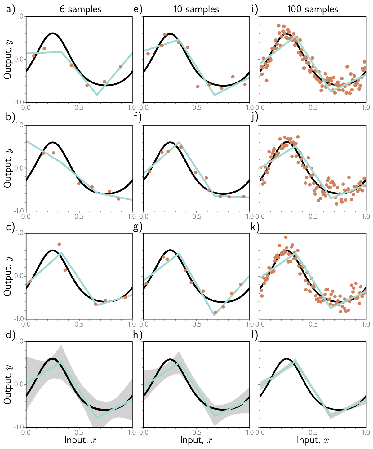
Variance comes from fitting limited, noisy data, so the remedy is more data. More examples average out the noise and sample the input space more densely. fig. 7 fits the three-region model to datasets of 6, 10, and 100 points. With six points the fit changes markedly from one dataset to the next; with 100 it barely changes. As a rule, adding training data almost always improves test performance. (Double descent will supply a strange exception.)
Prince §8.3.2, p. 125; figure on p. 127.
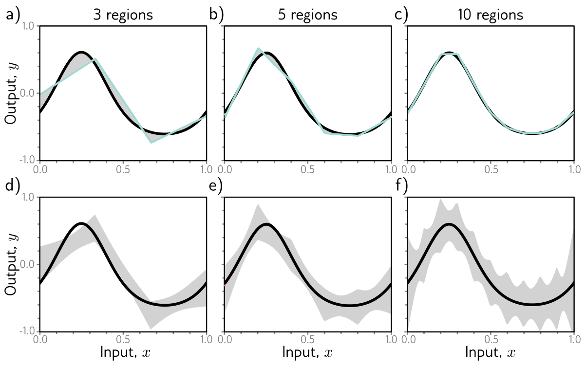
Bias comes from a model too inflexible to describe the true function, so the remedy is more capacity: for neural networks, more hidden units or more hidden layers. In the simplified model, more hidden units means more linear regions, and with ten regions the model can follow the true function closely (fig. 8a–c).
Prince §8.3.3, p. 125; figures on p. 128.
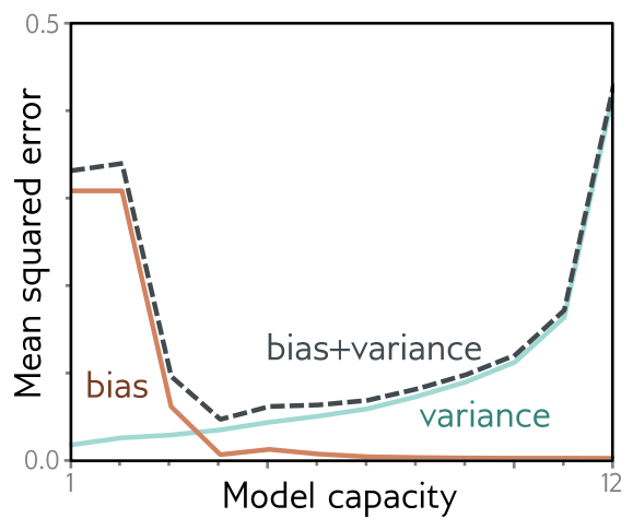
But look at fig. 8d–f. With the training-set size held fixed, the variance grows as the capacity grows. Adding capacity therefore does not necessarily reduce test error; it trades bias for variance. This is the bias–variance trade-off (Geman, Bienenstock, and Doursat 1992).
fig. 9 shows why. A three-region model fitted to three datasets of fifteen points gives nearly the same answer each time, because the noise roughly averages out within each region. A ten-region model fitted to the same three datasets fits each one better, so its training error is lower, but it spends much of its extra flexibility describing the noise. The fitted curves differ from one dataset to the next and are no closer to the truth. This is overfitting.
Since bias falls and variance rises with capacity, there should be an optimal capacity where their sum is smallest. fig. 10 computes both terms for the toy model with the data of fig. 9. The sum is minimized at a capacity of four: four hidden units, four linear regions.
Our version follows, with one addition. The optimum is not a property of the model alone; it depends on how much data there is.
    I  best D  bias + variance
   15       4           0.0088
   50       4           0.0032
  200       9           0.0012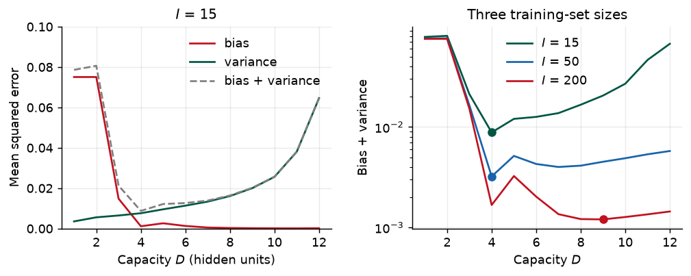
Prince, chapter notes, p. 134.
We have used capacity informally, to mean the number of hidden units or parameters. The notes sharpen it in two ways. The representational capacity is the set of functions the model can produce over all possible parameter values. The effective capacity is the smaller set an optimization algorithm can actually reach. More formal measures exist. The Vapnik–Chervonenkis (VC) dimension is the largest number of training examples a binary classifier can label in every possible way. The Rademacher complexity measures how well the model, with its parameters fitted optimally, can match random labels. The next section shows why counting parameters is a poor proxy for either.
Prince §8.4, pp. 127–129; figure on p. 130.
Does the bias–variance trade-off show up in practice? Prince returns to MNIST-1D, now with 10,000 training and 5,000 test examples, trains with Adam (step size 0.005, full batch, 4,000 steps), and steadily increases the number of hidden units in each of two hidden layers (fig. 12).
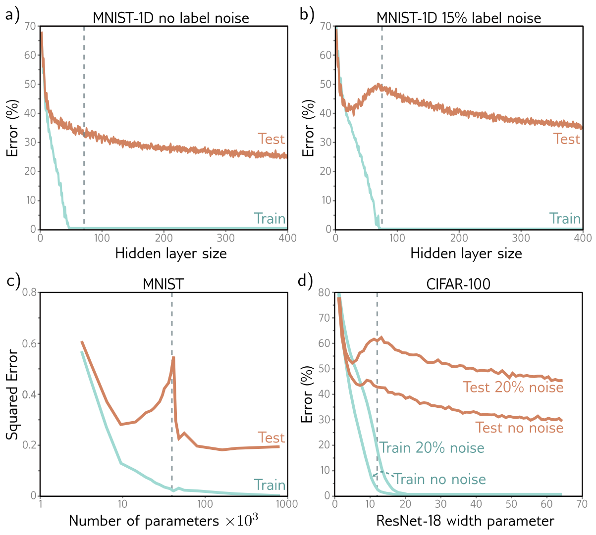
On the original data (panel a), the training error drops quickly to zero — well before the vertical dashed line where the parameter count equals the number of training examples. The test error, however, never turns up as the trade-off predicts. It just keeps decreasing.
Panel b repeats the experiment with 15% of the training labels randomized. Memorizing these noisier data takes almost as many parameters as there are data points. Now the test error does show the classical U: it falls, then rises as the model approaches the capacity at which it can fit the training data exactly. But then it does something unexpected. It falls again, and with enough capacity it ends below the minimum of the first U.
This is double descent (Belkin et al. 2019). It appears on unmodified MNIST (panel c). For other datasets, such as MNIST-1D and CIFAR-100 (panel d, from Nakkiran et al. (2021)), it appears or becomes more pronounced when label noise is added. The curve has three named regimes:
| Regime | Where | What happens to test error |
|---|---|---|
| Classical (under-parameterized) | Left of the peak | The bias–variance U |
| Critical | Near the point where training error first reaches zero | Rises to a peak |
| Modern (over-parameterized) | Right of the peak | Falls again, often below the classical minimum |
Prince §8.4.1, pp. 129–132; figures on pp. 131–132.
Double descent is recent, unexpected, and only partly understood. It is the combination of two effects. The first — test performance worsening when the model has just enough capacity to memorize the data — is exactly what the bias–variance trade-off predicts. The second is the puzzle: test performance keeps improving with capacity after training performance is already perfect, even though there are no longer enough data points to pin down the parameters uniquely.
Here is the key observation. Once the model can drive the training loss to near zero, extra capacity cannot help it fit the training data any better. Anything extra capacity changes must happen between the training points. A model’s tendency to prefer one solution over another as it fills in those gaps is its inductive bias.
What happens between the points matters a great deal, because in high dimensions the training data are extremely sparse. MNIST-1D has 40 input dimensions. Quantize each one into just 10 bins and there are \(10^{40}\) cells, against \(10^4\) training examples: on average one occupied cell in every \(10^{36}\). The way the volume of a high-dimensional space overwhelms any feasible amount of data is the curse of dimensionality.
Prince warns that the 1D and 2D pictures in the book should be treated with “healthy skepticism” (chapter notes, p. 135). In high dimensions, two random Gaussian vectors are nearly orthogonal; samples from a standard normal all sit at about the same distance from the origin, in a thin shell, even though the density is highest at the center (figure 8.13); almost all of a hypersphere’s volume lies next to its surface; and the nearest and farthest neighbors of a point are almost equally far away. Problems 8.6–8.9 ask for proofs, and the cell below checks the claims numerically.
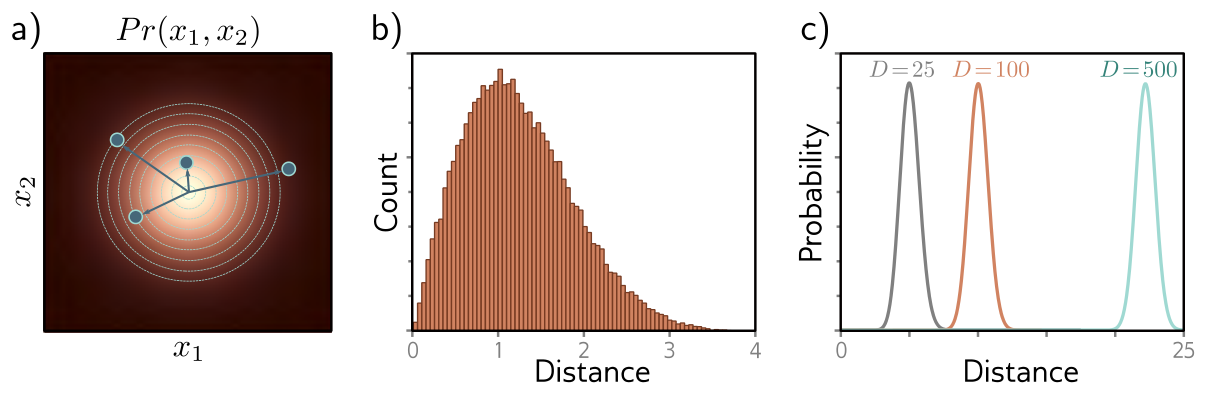
  dim  mean |x|  sd |x|  sqrt(dim)  mean |cos|  nearest/farthest
    2      1.24    0.67       1.41       0.637             0.009
   10      3.09    0.69       3.16       0.258             0.249
   40      6.24    0.68       6.32       0.127             0.533
  100      9.99    0.69      10.00       0.080             0.647
 1000     31.60    0.71      31.62       0.025             0.877
Read the columns from left to right. The distance from the origin grows like \(\sqrt{D}\), but its spread stays near 0.7 whatever the dimension: the samples live in a shell. The typical \(|\cos|\) between two random directions falls like \(1/\sqrt{D}\), so in 1,000 dimensions random vectors are within a couple of degrees of perpendicular. And the ratio of nearest to farthest distance climbs toward one, so “nearest neighbor” loses its meaning. At MNIST-1D’s 40 dimensions the nearest training example is already more than half as far away as the farthest.
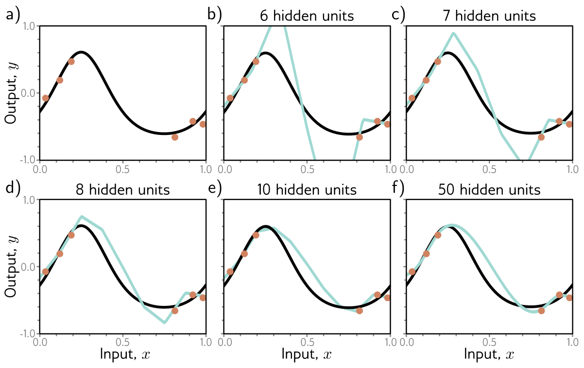
So real problems look like fig. 14a: small islands of data with wide gaps between them. The leading explanation of double descent is that, as we add capacity, the model interpolates between the data points more smoothly — and in the absence of any information about the gaps, smoothness is a sensible guess that tends to generalize. fig. 14b–f shows the smoothest function that passes through every data point, for an increasing number of hidden units. With barely enough parameters (panel b), the model must contort itself to hit every point, and its predictions between the points are erratic. That is why the peak of the double descent curve is so sharp. With more hidden units it can afford to be smooth.
That explains why big models can be smooth, not why they are. fig. 15 shows three functions the 50-unit model can produce, all of which pass exactly through the data and so have zero training loss. Something must steer training toward panel a rather than panels b or c.
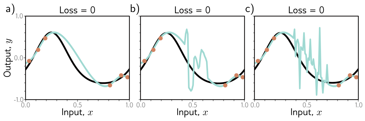
Prince offers two candidates. The initialization may start the network among smooth functions, and training may never leave them. Or the training algorithm may itself “prefer” smooth solutions. Anything that biases the solution toward some subset of equally good solutions is a regularizer, so the second possibility says the optimizer acts as an implicit regularizer — the starting point of Chapter 9.
For our simplified model, we can watch the second mechanism at work, because for a model that is linear in its parameters the implicit regularizer is known exactly. When \(D + 1 > I\), infinitely many parameter vectors fit the data perfectly. Gradient descent started from \(\boldsymbol{\phi} = \mathbf{0}\) only ever moves in directions spanned by the training feature vectors (each gradient is a combination of them), so it converges to the interpolating solution of minimum norm \(\|\boldsymbol{\phi}\|^2\). That is also the solution np.linalg.lstsq returns. In our model, the weight \(\omega_d\) is the change of slope at joint \(d\), so a small norm means the bending is spread thinly over many joints rather than concentrated in a few sharp kinks. In other words, the optimizer prefers smooth interpolants, and more joints give it more room to be smooth (Hastie et al. 2022).
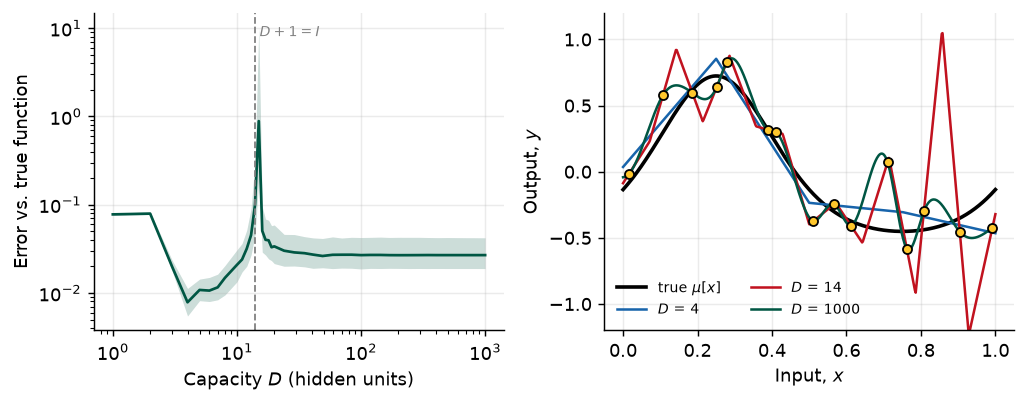
classical minimum: D = 4, error 0.0078
peak:              D = 15, error 0.8855
modern regime:     D = 1000, error 0.0268
The curve has all three regimes. Notice, though, that in this one-dimensional toy the second descent does not reach below the first: the over-parameterized model must still pass through every noisy point, and in one dimension the data leave no wide gaps for smoothness to exploit. Prince’s MNIST-1D and the CIFAR results sit in 40 and 3,072 dimensions, where nearly everything is gap. Double descent says that big models can generalize well; it does not promise that the biggest model always wins.
One more consequence is genuinely strange (chapter notes, pp. 134–135). Suppose a model sits in the modern regime and we add training data until the number of examples matches its capacity. Now the model sits at the peak of the new curve, and test performance can get worse. Nakkiran et al. also observe epoch-wise double descent: for a fixed model, test error can fall, rise, and fall again as training goes on. Effective capacity depends on the optimizer and the training time as well as on the architecture (Nakkiran et al. 2021).
Prince §8.5, pp. 132–133; chapter notes, pp. 135–136.
In the classical regime we cannot compute the bias (it needs the true function) or the variance (it needs many independent training sets). In the modern regime there is no way to know how much capacity to add before the test error stops improving. So in practice, how do we choose?
For a deep network, capacity depends on the number of hidden layers, the units per layer, and architectural choices still to come. The learning algorithm’s settings — learning rate, batch size, momentum, schedule — also affect test performance. All of these are hyperparameters. Finding good ones is hyperparameter search, or neural architecture search when the focus is on the network’s structure.
Hyperparameters are chosen empirically: train many models with different settings on the same training data, measure each one, keep the best. The crucial rule is where we measure them. Not on the test set. If we pick whichever settings score best on the test set, those settings might just happen to suit that particular test set, and the test score stops being an honest estimate of performance on new data. Instead we hold out a third dataset:
How much the test-set rule matters is easy to underestimate, so the cell below quantifies it. Imagine trying 50 hyperparameter settings that are, in truth, all equally good: each has a 25% error rate. Score them on a 200-example test set and report the best. Because each score is noisy, the best of 50 is mostly the luckiest of 50.
true error of every setting:                  0.250
reported error of the best of 50 (mean):       0.183
same model, scored on a fresh test set (mean): 0.249
chance the reported error is below 20%:       0.87
Reusing the test set to choose among 50 equally good models makes the winner look about 7 percentage points better than it is, and most of the time the report would claim an error under 20%. On a fresh test set the advantage vanishes, because there never was one. The same thing happens, more slowly, when a team tunes against a “test” set over months of experiments, or when a field tunes against a public benchmark over years.
The search itself is hard. Prince lists the reasons in the chapter notes (p. 135). Every evaluation means training a whole model, and the result is noisy, because training is stochastic. There are no gradients with respect to the hyperparameters. Many hyperparameters are discrete (the number of layers), and some are conditional (the width of layer 10 matters only if there are at least ten layers). And there are many local optima. The main strategies are these:
| Method | Idea | Notes |
|---|---|---|
| Grid search | Try every combination of a few values per hyperparameter | Cost explodes with the number of hyperparameters |
| Random search | Sample settings at random (Bergstra and Bengio 2012) | Beats a grid when only a few hyperparameters matter, since it tries many more distinct values of each |
| Bayesian optimization | Model validation performance and its uncertainty with a Gaussian process; pick the next setting to explore or exploit (Snoek, Larochelle, and Adams 2012) | Best for a few continuous hyperparameters |
| SMAC; Tree-Parzen estimators | Random-forest or density models that handle discrete and conditional choices | TPE models \(Pr(\text{hyperparameters} \mid \text{performance})\) instead |
| Hyperband | Start many random settings on a small budget; repeatedly keep the best fraction \(\eta\) and multiply the budget by \(1/\eta\) (Li et al. 2018) | Cheap, because bad settings are stopped early |
| BOHB | Hyperband with Tree-Parzen proposals instead of random ones | Combines both advantages |
The explore/exploit balance in Bayesian optimization is the bandit problem we met in Week 1’s reinforcement learning example, applied to choosing experiments.
Prince, chapter notes, p. 134; the industrial material is ours.
Splitting data three ways has a cost: every example in the validation or test set is one the model never trains on. When data are scarce — and in manufacturing, labeled defects usually are — a small training set means high variance.
\(k\)-fold cross-validation recovers some of that data. Merge the training and validation data and partition them into \(K\) disjoint folds. For each hyperparameter setting, train \(K\) times, each time holding out a different fold for validation and training on the other \(K - 1\), and average the \(K\) validation scores. Choose the setting with the best average. Prince describes estimating the final test performance by averaging the predictions of the \(K\) models on an entirely separate test set. Retraining one model on all the non-test data with the chosen setting is also common. Either way, the test set still plays no part in the choice.
Below, five-fold cross-validation chooses the capacity of the simplified model from a single dataset of 30 points, with no access to the truth. We then compare its choice with the truth, and repeat over 200 datasets to see how reliable it is.
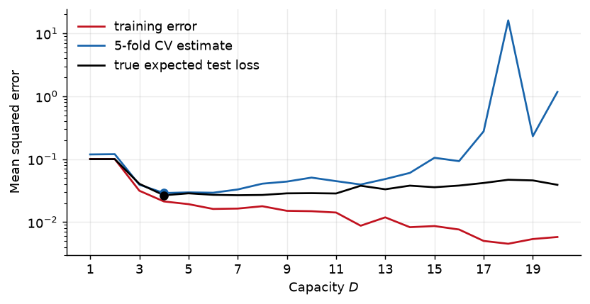
this dataset: CV chooses D = 4, the truth prefers D = 4
over 200 datasets: CV chooses D = 4 in 55% of them and D = 3 to 7 in 90%
median excess test error from CV's choice: 0.0006  (noise alone is 0.0225)
Cross-validation is not perfect — its choice wanders from dataset to dataset — but when it misses, it misses by little. That is the point: a model chosen honestly with slightly the wrong capacity is far better than one chosen dishonestly with an optimistic score.
Every split above assumes the examples are independent draws. Manufacturing data rarely are. Images from the same production lot share lighting, material, and fixture; sensor windows cut from the same machine run overlap in time; parts from the same supplier batch share defects. Split such data at random and nearly identical examples land on both sides of the split. The model is then tested on data it has effectively already seen, and the score is optimistic in exactly the way the cell above showed. Split by the unit you will deploy to — by lot, by machine, by week, by supplier — so that validation and test data come from units the model never trained on. scikit-learn’s GroupKFold and TimeSeriesSplit implement this.
Prince, chapter notes, p. 135.
Everything so far assumes the test data come from the same distribution as the data the model will meet after deployment. If they do not, the test score is not a guide to real-world performance. And the world drifts: a model that was accurate when deployed grows stale as the process changes. This is data drift, and it is why deployed models must be monitored. Prince names three ways it can happen (Moreno-Torres et al. 2012):
| Shift | What changes | Manufacturing example |
|---|---|---|
| Covariate shift | The input distribution \(Pr(\mathbf{x})\) | A new camera, or a second shift with different lighting, feeds the defect classifier images unlike any it trained on |
| Prior shift | The output distribution \(Pr(y)\) | A process improvement makes defects rare. A model that learned to call ambiguous parts “good” now misses most of the few defects there are, or, in reverse, floods inspectors with false alarms |
| Concept shift | The relationship \(Pr(y \mid \mathbf{x})\) | The customer tightens the tolerance, so parts that were “good” last month are now “defective” with the same measurements |
The practical response is the same in all three cases: keep a stream of labeled production data, recompute the error on it on a schedule, and treat a rise as a signal to retrain.
Prince §8.6, p. 133.
We measure performance on a separate test set. How well performance holds up on that set is generalization. Test error has three sources: noise, which nothing can remove; bias, from a model too inflexible to represent the truth; and variance, from fitting a particular, limited, noisy sample. For least squares regression they add exactly, eq. 7. More data reduces the variance. Below the point where the model can memorize the training data, more capacity reduces bias but increases variance — the bias–variance trade-off — and there is an optimal capacity, which grows with the amount of data.
Beyond that point the classical picture breaks. Test error can fall again as capacity increases even when the parameters outnumber the data, and the two effects together produce the double descent curve. The likely reason is that over-parameterized models, steered by an implicit regularizer in initialization or training, interpolate smoothly through the vast empty regions of a high-dimensional input space, although what exactly drives this is still unclear. To choose capacity and every other hyperparameter, we train candidate models, compare them on a validation set (or by \(k\)-fold cross-validation), and use the test set once, at the end. Even then, a test score speaks only for data drawn the way the test set was drawn.
Next: Chapter 9 turns the observation that “something steers training toward smooth solutions” into tools we control. Regularization — explicit penalties, early stopping, ensembling, dropout, data augmentation, and the implicit regularization of SGD itself — is how we reduce the variance term on purpose. Week 9 is also midterm week.
1. (UDL 8.1) Will the multiclass cross-entropy training loss in fig. 2 ever reach exactly zero? Explain your answer, and compare it with the final training loss printed under fig. 3.
2. (UDL 8.2 and 8.3*) Choose the first-layer weights and biases of the three-unit model of fig. 5a so that the hidden units respond as in panels b–d. Then show how the output parameters \(\{\beta, \omega_1,
\omega_2, \omega_3\}\) can be found in closed form under the least squares loss, and match your answer to the features and fit functions of the decomposition-check cell.
3. Fill in every step of eq. 6 from eq. 5. Which property of \(f_\mu[x]\) makes the cross term vanish? Then explain in a sentence each why the variance term cannot be estimated from one training set, and why the bias term cannot be estimated at all without knowing \(\mu[x]\).
4. (UDL 8.4) Consider the curve in fig. 12b at a hidden-layer size of 200, which has 50,410 parameters. What do you predict will happen to the training and test performance if the number of training examples rises from 10,000 to 50,410? Explain using the three regimes.
5. (UDL 8.5) Suppose the model capacity exceeds the number of training points and the model can drive the training loss to zero. What does this imply for fitting a heteroscedastic model, one that predicts its own noise variance (Week 5)? Propose a way to fix the problem you identify.
6. (UDL 8.6 and 8.9) Show that two random points drawn from a 1,000-dimensional standard normal distribution are nearly orthogonal, relative to the origin, with high probability. Then sample from standard normals in 25, 100, and 500 dimensions, plot histograms of the distances from the origin, and name the closed-form distribution they follow. Compare with the high-dimensions cell.
7. (UDL 8.7 and 8.8*) The volume of a hypersphere of radius \(r\) in \(D\) dimensions is \(\mathrm{Vol}[r] = r^D \pi^{D/2} / \Gamma[D/2 + 1]\). Use Stirling’s formula to show that the volume of a hypersphere of diameter one goes to zero as \(D\) grows. Then show that the fraction of a unit hypersphere’s volume lying in its outermost shell of thickness 0.01 goes to one.
8. Leakage on the line. A team trains a CNN to detect weld defects from images collected across 40 production lots. A random 80/10/10 split gives 96% test accuracy, but the first new lot after deployment scores 78%. (a) Explain the gap using the leakage callout above. (b) Design a split that would have predicted the 78%. (c) Which of the three dataset shifts could also contribute, and what would you monitor to tell them apart?
9. Classify the drift. A predictive-maintenance model flags spindle bearings likely to fail within 100 hours. For each event, name the shift (covariate, prior, or concept) and say whether retraining on recent data alone is enough: (a) the plant switches to a bearing supplier whose vibration signatures run hotter; (b) a new preventive-maintenance policy makes failures half as frequent; (c) “failure” is redefined from seizure to any vibration level above an ISO threshold.
10. Computational. In the fig-double-descent cell, replace the minimum-norm solution with ridge regression, \(\boldsymbol{\phi} =
(\mathbf{X}^T\mathbf{X} + \lambda\mathbf{I})^{-1}\mathbf{X}^T\mathbf{y}\), for \(\lambda \in \{10^{-6}, 10^{-3}, 10^{-1}\}\). What happens to the peak? Then return to \(\lambda = 0\) and draw the \(x_i\) uniformly over \([0, 1]\) instead of one per segment. Does the peak move or change height? (This previews Chapter 9.)
11. Computational. Extend the winners-curse cell. (a) Plot the mean optimism, true error minus reported error, against the number of settings tried (1 to 500) for test sets of 200, 1,000, and 10,000 examples. (b) Give a rough formula: the optimism should scale like the standard error \(\sqrt{p(1-p)/n}\) times a factor that grows slowly with the number of settings. Which factor?
12. Computational. Return to fig. 3. Hold out 100 of the 400 training examples as a validation set, train on the other 300, and stop training at the step with the lowest validation loss. Report the test error and test loss at that step and compare them with the final values. This is early stopping, the first regularizer of Chapter 9.
Every part of this page, mapped to Prince, Understanding Deep Learning (MIT Press, 2024) (Prince 2024). Page numbers are those of the printed book.
| This page | Prince section | Pages | Figures used |
|---|---|---|---|
| A Trained Model Is Not Yet a Good Model | Ch. 8 opening | 118 | — |
| Training a Simple Model | §8.1 | 118–120 | 8.1, 8.2 (p. 119) |
| Sources of Error | §8.2 | 120–122 | 8.3 (p. 120), 8.4 (p. 121) |
| — Noise, bias, and variance | §8.2.1 | 122–123 | 8.5 (p. 122) |
| — Mathematical formulation of test error | §8.2.2; notes | 123–124, 133–134 | — |
| Reducing Error | §8.3 | 124–125 | — |
| — Reducing variance | §8.3.1 | 125 | 8.6 (p. 126) |
| — Reducing bias | §8.3.2 | 125 | 8.7 (p. 127) |
| — The bias–variance trade-off | §8.3.3 | 125 | 8.8, 8.9 (p. 128) |
| — What “capacity” means | notes | 134 | — |
| Double Descent | §8.4 | 127–129 | 8.10 (p. 130) |
| — Explanation | §8.4.1; notes | 129–132, 134–135 | 8.11 (p. 131), 8.12 (p. 132), 8.13 (p. 137) |
| Choosing Hyperparameters | §8.5; notes | 132–133, 135–136 | — |
| Cross-Validation in Practice | notes; ours | 134 | — |
| When the Test Set Is Not the World | notes | 135 | — |
| Summary | §8.6 | 133 | — |
| Exercises 1, 2, 4–7 | Problems 8.1–8.9 | 136–137 | — |
Equations on this page correspond to Prince as follows: eq. 1 is his (8.1), eq. 2 is (8.2), eq. 3 is (8.3), eq. 4 is (8.4), eq. 5 is (8.5), eq. 6 is (8.6), and eq. 7 is (8.7). The hypersphere volume in exercise 7 is his (8.8).
Figures 8.1–8.13 are reproduced unaltered from Prince, Understanding Deep Learning (MIT Press, 2024), which is distributed under a Creative Commons CC-BY-NC-ND license, and are used here for non-commercial classroom instruction. Original sources credited within the figures: figure 8.1 is adapted from Greydanus (2020); figure 8.10c shows results from Belkin et al. (2019) and figure 8.10d results from Nakkiran et al. (2021). All other figures on this page are generated by the code in this week’s notebook.