Input dimensions (224 x 224 x 3)                   150,528
Fully connected layer, width D_in           22,658,829,312 parameters  (91 GB in float32)
3x3 convolution, 3 -> 64 channels                    1,792 parameters
Ratio 12,644,436 : 1Convolutional and Residual Networks
Weeks 10–11 · Sessions 20–21 · October 29 & November 3, 2026
architectures
Why images need their own layers: invariance and equivariance, the convolution operation in 1D and 2D, padding, stride, dilation, channels, receptive fields, pooling and upsampling, the classic ImageNet architectures, and then residual connections and batch normalization — the two ideas that let convolutional networks grow from eight layers to hundreds.
How to read the references in these notes
Every section below opens with the section number and page range it covers in Prince, Understanding Deep Learning (MIT Press, 2024). Page numbers are those of the printed book. Figures taken from the textbook are captioned with their original figure number and page; figures generated by the code behind this page are ours. A complete cross-reference table appears in Section 12.
1 Learning Objectives
By the end of these two sessions you should be able to:
- State the three properties of images that make fully connected networks a poor fit, and define invariance and equivariance to a transformation.
- Write the 1D and 2D convolution operations, and compute the output size of a convolutional layer from its kernel size, stride, padding, and dilation.
- Explain why a convolutional layer is a fully connected layer with a sparse, repeated weight matrix, count the parameters of a layer with \(C_i\) input and \(C_o\) output channels, and compute receptive fields through a stack of layers.
- Describe the three ways to downsample a representation and the four ways to upsample it, and explain what a 1×1 convolution does.
- Trace an image through AlexNet and VGG, and say what the output of an object detector and a semantic segmentation network looks like.
- Explain the shattered gradients conjecture for why very deep sequential networks fail to train, and how residual connections turn a deep network into an ensemble of shallow paths.
- Show why activations in a residual network grow exponentially with depth, and how batch normalization replaces that with linear growth; state what BatchNorm computes at training and at test time.
- Sketch the ResNet, bottleneck, DenseNet, and U-Net blocks, and build and train a small convolutional classifier in PyTorch.
The code lives in a notebook
This page shows the figures and results; except in the PyTorch section near the end, the Python behind them is not printed here. All of it — every cell, in the order the note uses it — is in a notebook you can open in the browser with nothing to install:
- ▶ Open the Week 10 notebook in Google Colab — all of this page’s code, in order.
- ▶ UDL notebook 10.1 — 1D convolution — build the weight matrices of fig. 5 by hand.
- ▶ UDL notebook 10.2 — Convolution for MNIST-1D — the experiment of fig. 11.
- ▶ UDL notebook 10.3 — 2D convolution — fig. 13 and fig. 14 in code.
- ▶ UDL notebook 10.4 — Downsampling and upsampling — fig. 16 to fig. 19.
- ▶ UDL notebook 10.5 — Convolution for MNIST — a 2D convolutional classifier on real digit images.
- ▶ UDL notebook 11.1 — Shattered gradients — the experiment behind fig. 31.
- ▶ UDL notebook 11.2 — Residual networks — the variance growth of fig. 35.
- ▶ UDL notebook 11.3 — Batch normalization — the forward and backward pass of eq. 15 to eq. 17.
Colab gives you a Python environment with NumPy, matplotlib, and PyTorch already installed. In Colab, run a cell with Shift+Enter. If you prefer to work locally, pip install -r requirements.txt from the course repository gives you the same environment.
2 Why Images Need Their Own Layers
Prince, Chapter 10 opening, p. 161.
Every network so far has been fully connected: each hidden unit sees every input, and there is a single path from input to output. Chapters 10 to 13 introduce components with sparser connections, shared weights, and parallel paths, and this chapter’s component — the convolutional layer — is the one built for images. Prince gives three reasons a fully connected network is the wrong tool for an image.
- Images are high-dimensional. A 224×224 RGB image has 150,528 input values. Hidden layers are usually at least as wide as the input, so one fully connected layer would need more than \(150{,}528^2 \approx 22\) billion weights.
- Nearby pixels are related. A fully connected network has no notion of “nearby”. If you permuted the pixels of every training and test image in the same way, it would train exactly as well. Convolution builds the neighborhood structure in.
- The interpretation is stable under geometric transformations. A photo of a tree shifted three pixels to the left is still a tree, but every input to a fully connected network has changed, so it must learn the pattern “tree” separately at every position.
A convolutional layer processes each local region with the same parameters, shared across the whole image. It therefore has far fewer parameters, exploits the spatial relationships between pixels, and learns each pattern once. A network built mostly from such layers is a convolutional neural network (CNN). The first cell makes the parameter argument concrete.
The convolutional layer’s parameter count does not depend on the image size at all. It would be the same 1,792 for a 4K frame from an inspection camera. That is the practical reason CNNs took over computer vision, and the rest of this chapter explains the structural one.
3 Invariance and Equivariance
Prince §10.1, pp. 161–162; figure on p. 162.
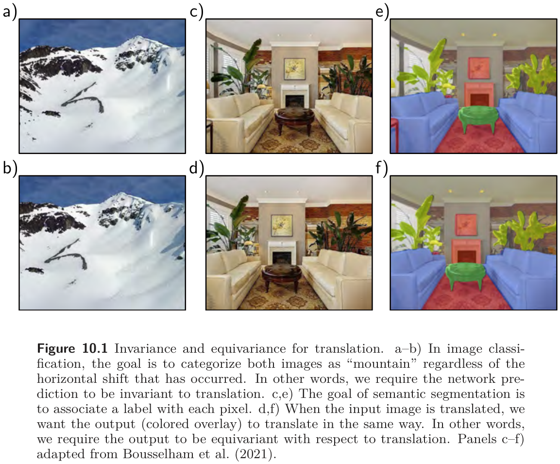
Saying that “a tree is still a tree after a shift” can be made precise. A function \(f[\mathbf{x}]\) of an image \(\mathbf{x}\) is invariant to a transformation \(t[\mathbf{x}]\) if
\[ f\big[t[\mathbf{x}]\big] = f[\mathbf{x}], \tag{1}\]
so the output is the same whether or not the transformation was applied. An image classifier should be invariant to translation, rotation, flips, and mild warps (fig. 1a–b). A function is equivariant (or covariant) to the transformation if
\[ f\big[t[\mathbf{x}]\big] = t\big[f[\mathbf{x}]\big], \tag{2}\]
so the output changes in the same way as the input. A segmentation network, which labels every pixel, should be equivariant: shift the image and the label map should shift with it (fig. 1c–f).
Convolutional layers are equivariant to translation by construction, and the pooling operations of Section 6 add partial invariance. The next cell checks both properties on a 1D signal, and shows that a fully connected layer has neither.
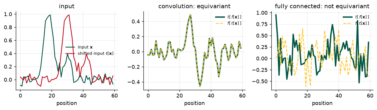
operation                                           max |difference|
convolution, f[t[x]] vs t[f[x]]                             0.00e+00
fully connected, f[t[x]] vs t[f[x]]                         9.31e-01
convolution + global max pool, f[t[x]] vs f[x]              0.00e+00
Notation
Prince writes a vector input as \(\mathbf{x}\) with elements \(x_i\), the kernel as \(\boldsymbol{\omega}\) with elements \(\omega_j\), a layer’s output as \(\mathbf{z}\) before the activation and \(\mathbf{h}\) after it, and the activation function as \(\mathrm{a}[\bullet]\). A 2D input is a matrix \(\mathbf{X}\) with elements \(x_{ij}\); a stack of channels is a 3D tensor. A kernel is also called a filter, and a channel a feature map. Square brackets denote function application throughout.
4 Convolutional Networks for 1D Inputs
Prince §10.2, pp. 163–170.
Convolutional networks consist of a series of convolutional layers, each equivariant to translation, usually with pooling in between to induce partial invariance. Prince develops everything in 1D first, where it can be drawn, and then lets the 2D case follow in one step.
4.1 The 1D convolution operation
Prince §10.2.1, p. 163; figure on p. 163.
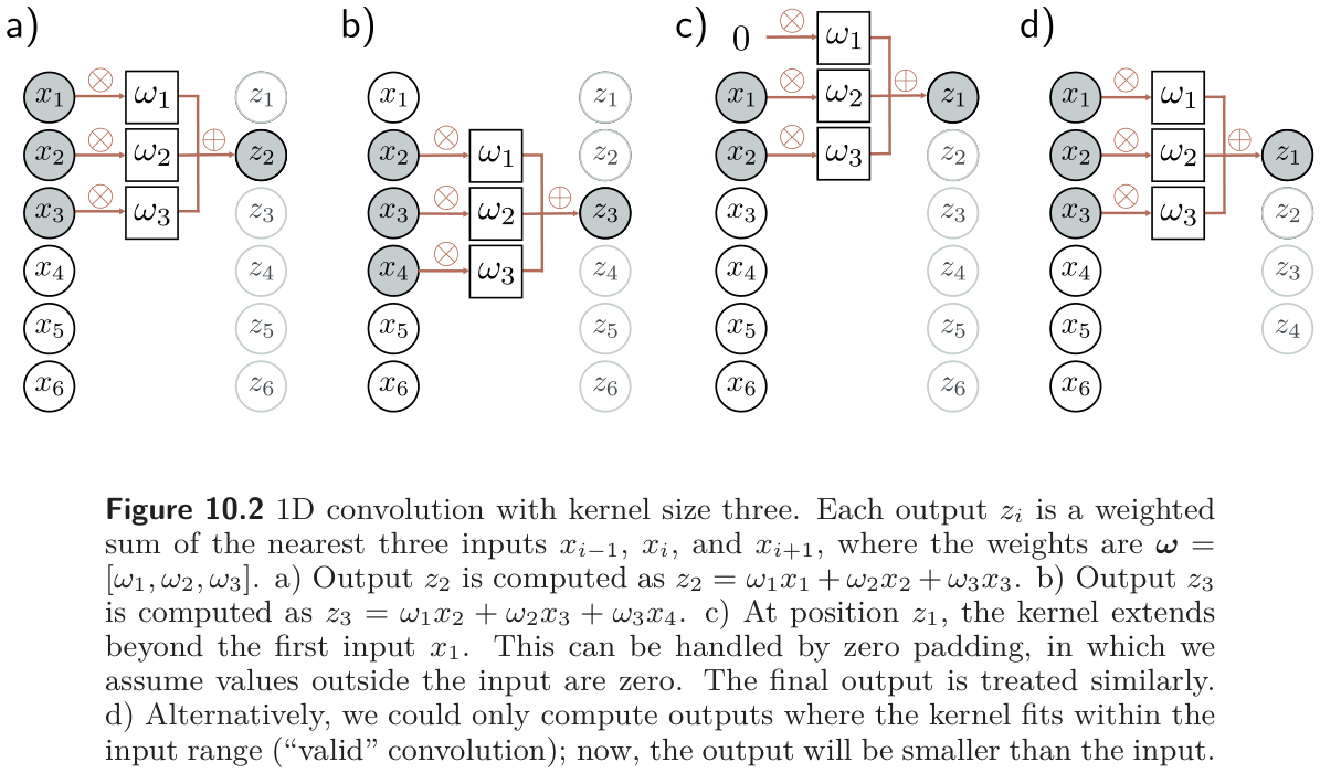
A 1D convolution turns an input vector \(\mathbf{x}\) into an output vector \(\mathbf{z}\) in which every output is a weighted sum of nearby inputs, with the same weights at every position. The weights are the convolution kernel (or filter), and the number of inputs combined is the kernel size. For kernel size three,
\[ z_i = \omega_1 x_{i-1} + \omega_2 x_i + \omega_3 x_{i+1}, \tag{3}\]
where \(\boldsymbol{\omega} = [\omega_1, \omega_2, \omega_3]^T\) (fig. 3). Shift the input by one position and every \(z_i\) moves with it, which is exactly the equivariance we just checked numerically.
Strictly, this is cross-correlation
In signal processing, a convolution flips the kernel: it would pair \(\omega_1\) with \(x_{i+1}\) and \(\omega_3\) with \(x_{i-1}\). Equation eq. 3 is a cross-correlation. Machine learning calls it a convolution anyway, because the kernel is learned and the flip is immaterial, and every deep learning library (torch.nn.Conv1d included) follows that convention. Prince notes this in a footnote on p. 163.
Worked: convolution is translation-equivariant (problem 10.1)
Let \(t[\mathbf{x}]\) shift the input by one position, so the new input is \(x'_i = x_{i-1}\). Apply eq. 3 to it: \[ z'_i = \omega_1 x'_{i-1} + \omega_2 x'_i + \omega_3 x'_{i+1} = \omega_1 x_{i-2} + \omega_2 x_{i-1} + \omega_3 x_{i} = z_{i-1}. \] The output is the original output shifted by the same amount: \(f[t[\mathbf{x}]] = t[f[\mathbf{x}]]\). The argument uses only that the same weights appear at every position, which is why it fails for a fully connected layer, where eq. 6 below gives each position its own weights.
4.2 Padding
Prince §10.2.2, p. 164.
Equation eq. 3 needs \(x_{i-1}\) for the first output and \(x_{i+1}\) for the last, and neither exists. There are two conventions. Zero padding treats the input as zero outside its range (fig. 3c); other choices wrap the signal around or reflect it at the ends. A valid convolution instead computes only the outputs where the kernel fits entirely inside the input (fig. 3d). Valid convolution invents no values at the edges, but the representation shrinks by \(K - 1\) positions per layer, which is why most modern networks pad.
4.3 Stride, kernel size, and dilation
Prince §10.2.3, pp. 164–165; figure on p. 164.
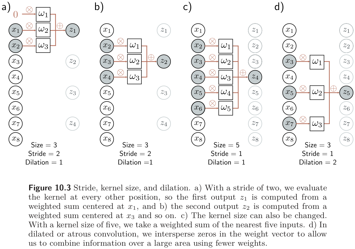
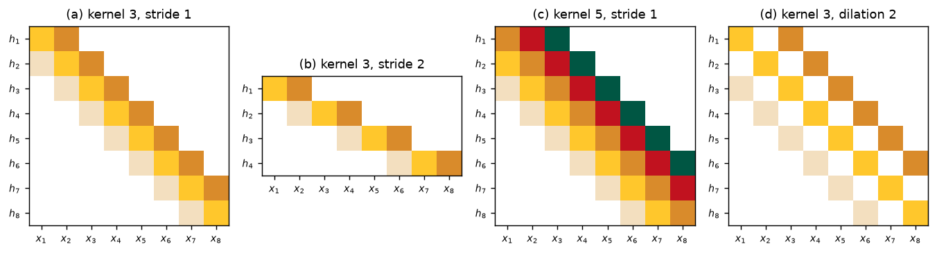
Equation eq. 3 is one member of a family. The stride is how far the kernel moves between outputs; with stride two there are roughly half as many outputs as inputs (fig. 4a–b). The kernel size can grow to integrate over a wider region (fig. 4c), and it is usually odd so that the kernel is centered on the current position; the cost is more weights. A dilated (or atrous) convolution gets a wide view without the weights by interspersing zeros in the kernel: a kernel of size five with its second and fourth entries fixed at zero covers five positions with three parameters (fig. 4d). The number of zeros between weights sets the dilation rate.
The book does not state the output-size formula, but you will use it constantly. For an input of length \(D\), kernel size \(K\), stride \(s\), padding \(p\) on each side, and dilation \(d\), the number of outputs is
\[ D_{\text{out}} = \left\lfloor \frac{D + 2p - d\,(K-1) - 1}{s} \right\rfloor + 1, \tag{4}\]
where \(d\,(K-1) + 1\) is the effective kernel size. The cell checks the formula against PyTorch for the network of fig. 10 and a few other settings.
setting                                          D_in  formula  PyTorch
figure 10.7, layer 1  (valid, stride 2)            40       19       19
figure 10.7, layer 2                               19        9        9
figure 10.7, layer 3                                9        4        4
kernel 3, 'same' zero padding                      40       40       40
kernel 3, stride 2, zero padding                   40       20       20
kernel 3, dilation 2, padding 2                    40       40       40
kernel 7, dilation 3, stride 3 (problem 10.4)      40        8        8
4.4 Convolutional layers
Prince §10.2.4, p. 165; figure on p. 166.
A convolutional layer convolves the input, adds a bias \(\beta\), and passes the result through an activation function. With kernel size three, stride one, and dilation one, the \(i\)th hidden unit is
\[ h_i = \mathrm{a}\big[\beta + \omega_1 x_{i-1} + \omega_2 x_i + \omega_3 x_{i+1}\big] = \mathrm{a}\Big[\beta + \sum_{j=1}^{3} \omega_j\, x_{i+j-2}\Big], \tag{5}\]
with zero padding where the index runs off the end. Compare the fully connected layer of Chapter 4,
\[ h_i = \mathrm{a}\Big[\beta_i + \sum_{j=1}^{D} \omega_{ij}\, x_j\Big]. \tag{6}\]
With \(D\) inputs and \(D\) hidden units, eq. 6 has \(D^2\) weights and \(D\) biases; eq. 5 has three weights and one bias. The convolutional layer is a special case of the fully connected one: set most of the weights in \(\boldsymbol{\Omega}\) to zero and constrain the rest to repeat along the diagonals (fig. 5). A fully connected network can therefore represent anything a convolutional network can. Whether it finds that solution is the question Section 4.7 answers.
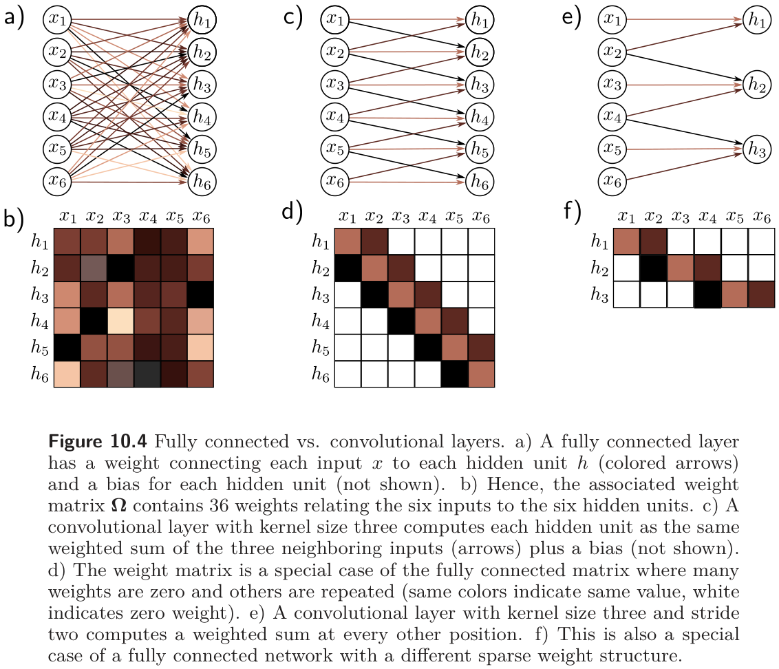
The next figure builds the weight matrices of fig. 5d and fig. 5f directly, by pushing each basis vector \(\mathbf{e}_j\) through conv1d and reading off a column. It also answers problem 10.5 for the kernel-five and dilated cases.
4.5 Channels
Prince §10.2.5, pp. 165–167; figure on p. 166.
A single convolution loses information: it averages neighbors, and the ReLU clips everything negative. So several convolutions are computed in parallel, each with its own kernel and bias, and each producing its own set of hidden units called a channel or feature map (fig. 7a–b). The hidden layer is then a 2D array \(\mathbf{H}_1\) of positions × channels. The next layer’s kernels take a weighted sum over all input channels at the nearest \(K\) positions (fig. 7c).
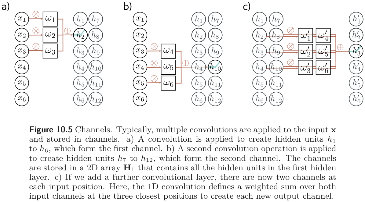
The parameter count follows directly. If the incoming layer has \(C_i\) channels, the kernel size is \(K\), and there are \(C_o\) output channels, each output channel needs a weight for every (input channel, kernel position) pair plus one bias, so the layer has
\[ \boldsymbol{\Omega} \in \mathbb{R}^{C_i \times C_o \times K} \quad\text{weights and}\quad \boldsymbol{\beta} \in \mathbb{R}^{C_o} \quad\text{biases}, \tag{7}\]
a total of \(C_i C_o K + C_o\) parameters, and in 2D \(C_i C_o K^2 + C_o\). The cell checks the formula against nn.Conv1d and nn.Conv2d for the layers in problems 10.8 and 10.14.
layer                                                       weights  biases  PyTorch
1D, 3 -> 4 channels, kernel 3    (problem 10.8, layer 1)         36       4       40
1D, 4 -> 10 channels, kernel 5   (problem 10.8, layer 2)        200      10      210
2D, 3 -> 10 channels, kernel 5x5 (problem 10.14)                750      10      760
2D, 3 -> 64 channels, kernel 3x3                              1,728      64    1,792
4.6 Receptive fields
Prince §10.2.6, p. 167; figure on p. 168.
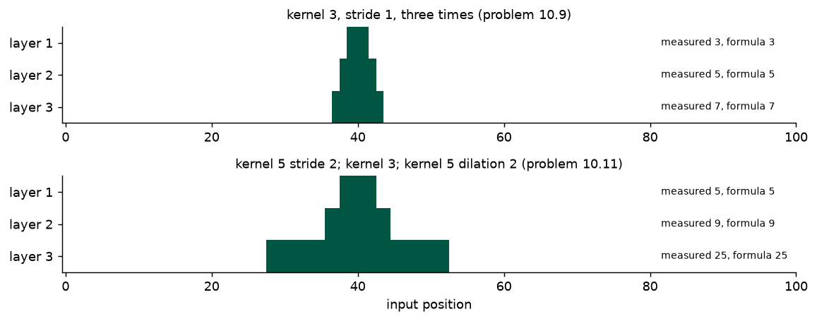
The receptive field of a hidden unit is the region of the original input that feeds into it. With kernel size three, a unit in the first layer sees three inputs. A unit in the second layer sees three first-layer units, each of which sees three inputs, so its receptive field is five. Each layer adds two, and information from across the input is integrated gradually (fig. 8). Stride accelerates this: after a stride-two layer, every later kernel position is two input positions apart, so the same kernel covers twice the input.
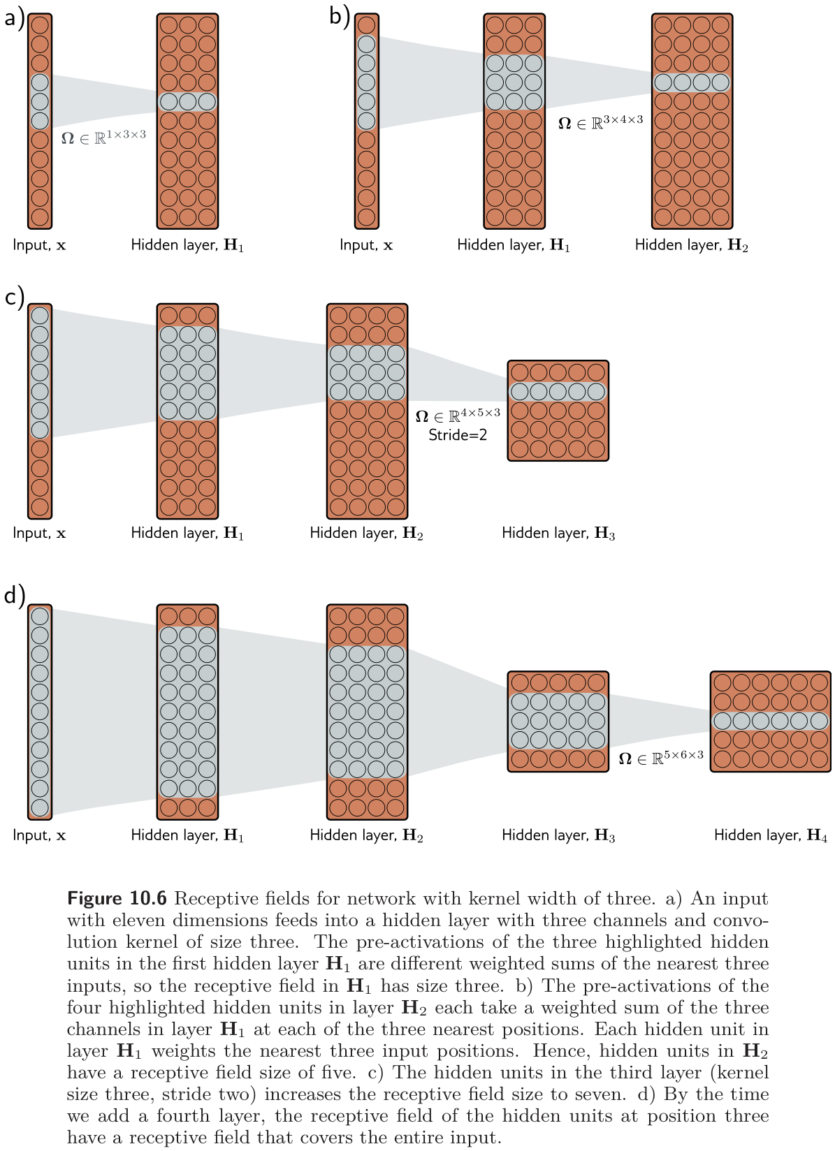
The general rule, which is not in the book but is worth having, is that layer \(\ell\) with kernel size \(K_\ell\) and dilation \(d_\ell\) enlarges the receptive field by
\[ R_\ell = R_{\ell-1} + d_\ell\,(K_\ell - 1) \prod_{m<\ell} s_m, \qquad R_0 = 1, \tag{8}\]
where the product of the earlier strides is the spacing, in input positions, between adjacent units of layer \(\ell - 1\). The cell measures receptive fields empirically — by differentiating one output unit with respect to the input and seeing which inputs have nonzero gradient — and compares with eq. 8 for the two networks in problems 10.9 and 10.11.
4.7 Example: MNIST-1D
Prince §10.2.7, pp. 167–170; figures on p. 169.
Prince’s running example from Week 8 returns. The MNIST-1D input is a 40-dimensional vector and the output a 10-dimensional vector of class activations. fig. 10 is the network: three convolutional layers, each with fifteen channels, kernel size three, stride two, and valid padding, so the representation shrinks 40 → 19 → 9 → 4 positions (exactly as the shape calculator above computed), then the 4×15 = 60 hidden units are flattened and mapped by a fully connected layer to the ten outputs.
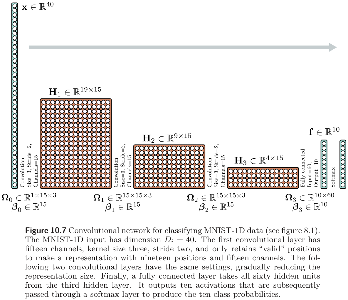
The comparison network is fully connected with the same number of layers and hidden units per layer — 285, 135, and 60. The convolutional network has 2,050 parameters; the fully connected one has 59,065. Both fit the training data perfectly, but the convolutional network reaches about 17% test error and the fully connected network about 40% (fig. 11).
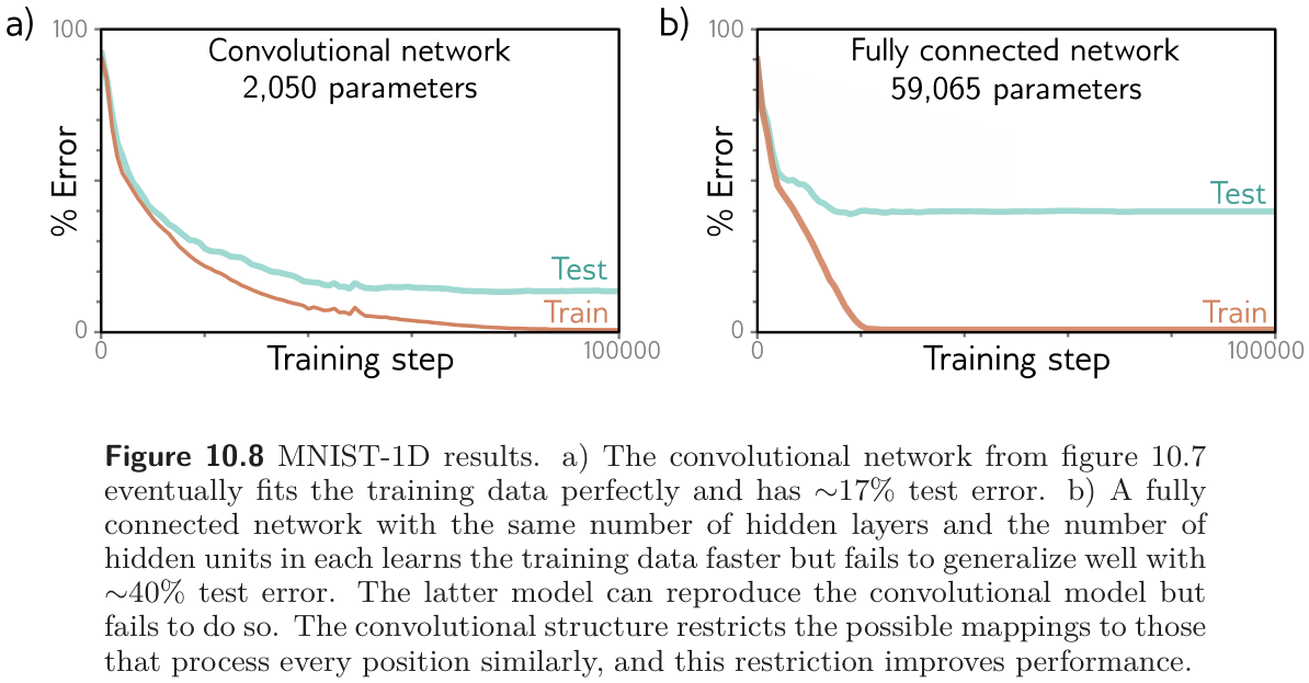
The explanation is not the parameter count — Chapter 8 showed that overparameterization generally helps. The fully connected network could reproduce the convolutional one exactly (fig. 5) and fails to. The convolutional architecture has a better inductive bias: we know the data were generated by translating a template, so forcing every position to be processed the same way restricts the search to a smaller family of plausible mappings. Prince offers two equivalent readings. The convolutional network searches a smaller family of input-to-output functions, all of which are plausible; or, the convolutional structure is a regularizer that applies an infinite penalty to most of the solutions the fully connected network can express. Either way it is the Week 9 story — a prior over functions — built into the architecture rather than added to the loss.
We can run the experiment ourselves. The cell generates an MNIST-1D-style dataset (ten fixed templates, randomly stretched, randomly placed in a 40-sample window, plus noise), builds both networks with exactly the parameter counts above, and trains them with SGD.
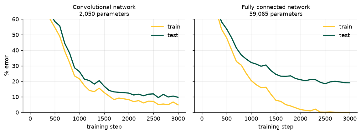
Convolutional network      final train error   4.8%   final test error   9.7%
Fully connected network    final train error   0.0%   final test error  19.0%
5 Convolutional Networks for 2D Inputs
Prince §10.3, pp. 170–171; figures on pp. 171–172.
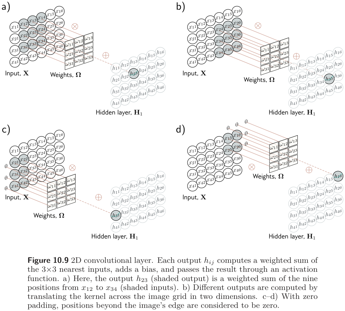
1D convolutional networks are used for audio, financial time series, text, and — in the manufacturing literature — vibration and current signals for bearing and tool-wear diagnosis. But the main use of convolution is on images, and the step from 1D to 2D is only notational. A 3×3 kernel \(\boldsymbol{\Omega} \in \mathbb{R}^{3\times 3}\) applied to an input with elements \(x_{ij}\) gives
\[ h_{ij} = \mathrm{a}\Big[\beta + \sum_{m=1}^{3}\sum_{n=1}^{3} \omega_{mn}\, x_{i+m-2,\; j+n-2}\Big], \tag{9}\]
a weighted sum over a square 3×3 region, with the kernel translated both horizontally and vertically across the input (fig. 13).
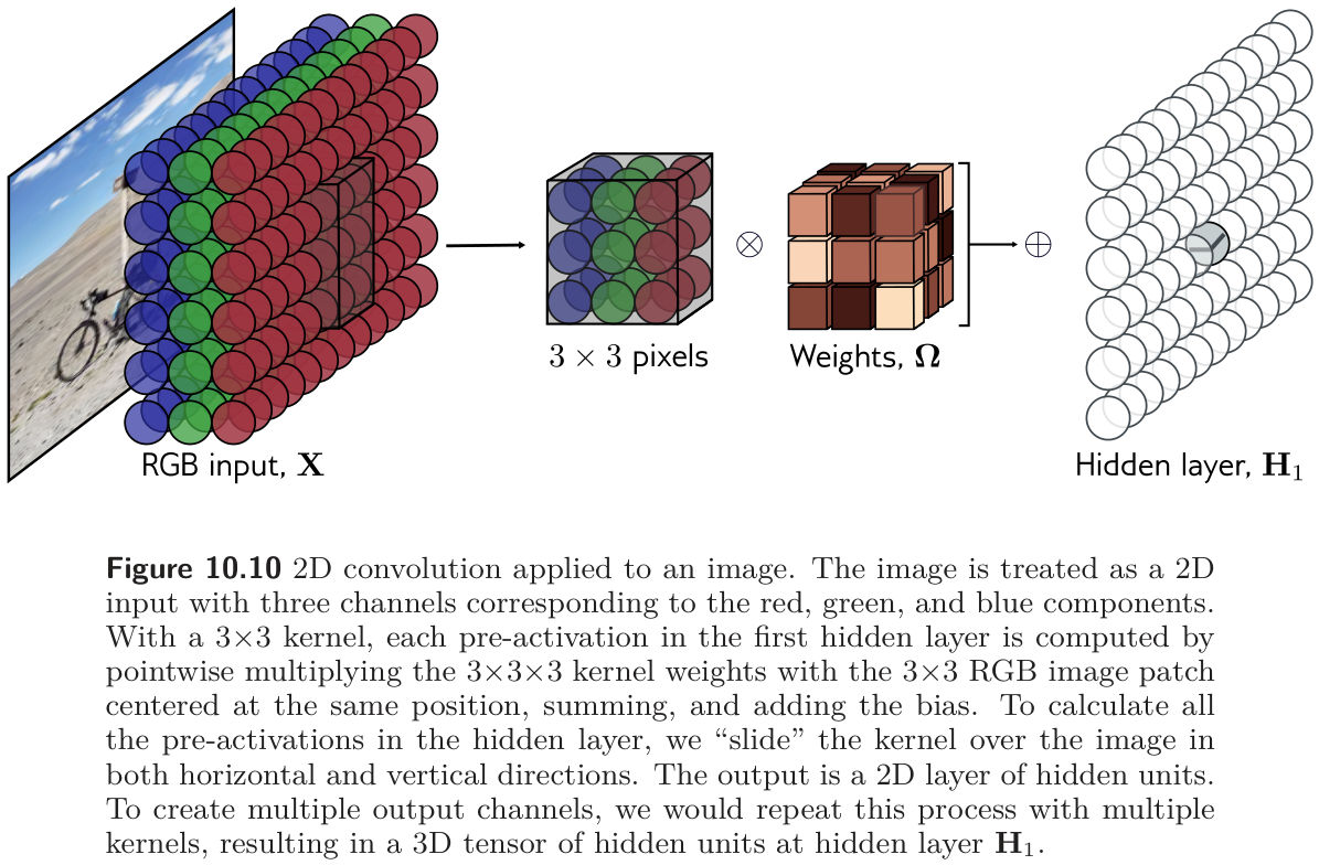
An RGB image is a 2D signal with three channels, so a 3×3 kernel on it has 3×3×3 weights, applied at every position to produce one 2D output channel the same size as the input (with zero padding). More output channels come from more kernels, stacked into a 3D tensor (fig. 14). In general, with kernel size \(K \times K\), \(C_i\) input channels, and \(C_o\) output channels, each output channel is a weighted sum of \(C_i \times K \times K\) quantities plus a bias, so the layer has \(C_i C_o K^2\) weights and \(C_o\) biases — the 2D form of eq. 7, which the parameter-count cell above already verified.
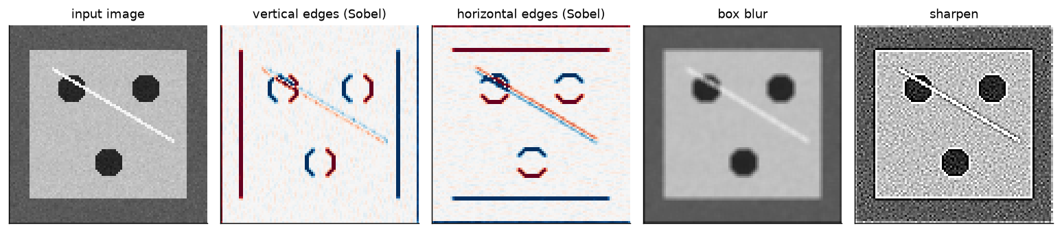
Before the kernels are learned, it helps to see what hand-designed ones do. The cell builds a synthetic inspection image — a bright machined plate on a darker background with three bolt holes and a thin diagonal scratch — and convolves it with four classic 3×3 kernels.
6 Downsampling and Upsampling
Prince §10.4, pp. 171–174; figures on pp. 173–175.
The network of fig. 10 grew its receptive fields by shrinking the representation with stride-two convolutions. This section collects the ways to scale a 2D representation down (downsampling), scale it back up (upsampling, needed when the output is itself an image), and change the number of channels without touching the spatial size.
6.1 Downsampling
Prince §10.4.1, pp. 171–172; figure on p. 173.
There are three common ways to halve each spatial dimension (fig. 16). Subsampling keeps every other position; a stride-two convolution does this implicitly, without ever computing the discarded values (panel a). Max pooling keeps the maximum of each 2×2 block (panel b). It induces some invariance to translation: shift the input by one pixel and many of the maxima are unchanged. Mean (or average) pooling averages each block (panel c). All three act on each channel separately, so the output has half the width and height and the same number of channels.
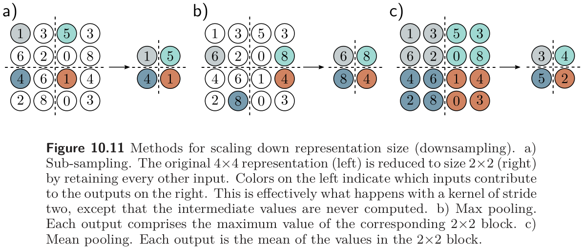
The cell tests the invariance claim on the kind of map pooling usually sees: the sparse output of a detector, a few sharp peaks where some feature was found and near-zero elsewhere. It shifts the map by one pixel, pools both versions, and measures two things: how much the pooled map changes, and how much of each peak’s height survives pooling.
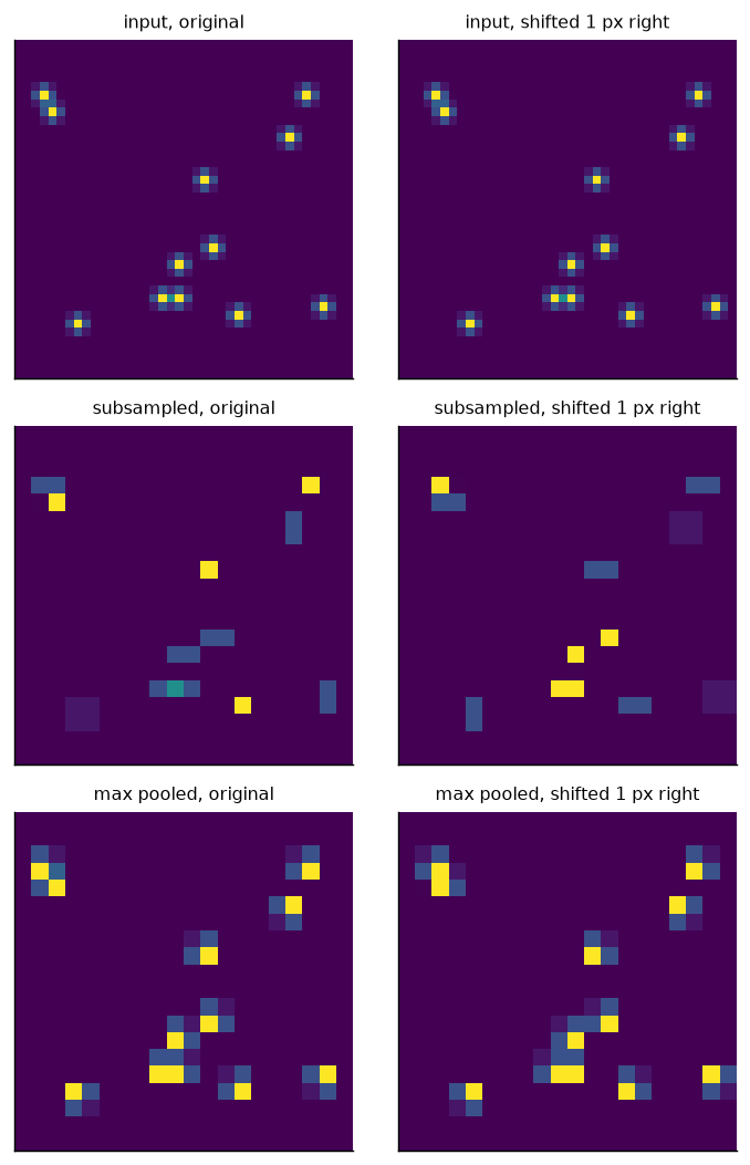
downsampling    change in pooled map   peak height kept (mean)  (worst)
subsample                        98%                       46%       6%
max pool                         73%                      100%     100%
mean pool                        76%                       41%      39%
The table supports a modest version of Prince’s claim. A one-pixel shift still changes all three pooled maps, so pooling only gives partial invariance. But max pooling changes the map least, and it is the only method that never loses a detection. Every peak survives at full height. A sharp feature that falls between the sample points of subsampling can vanish altogether, and mean pooling dilutes it.
6.2 Upsampling
Prince §10.4.2, pp. 172–174; figures on p. 173.
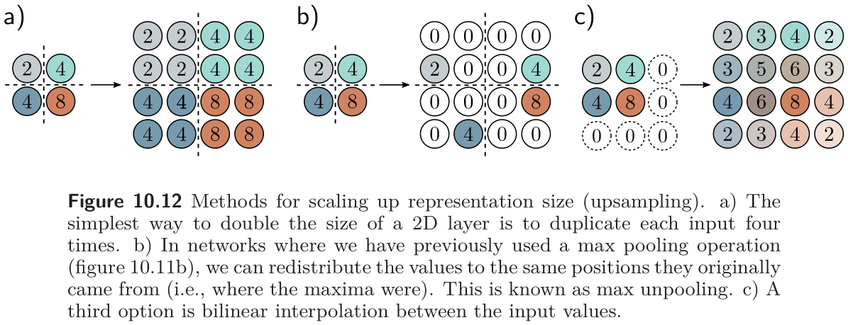
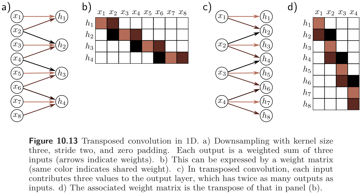
Four ways to double the resolution (fig. 18 and fig. 19). The simplest duplicates every value into a 2×2 block. Max unpooling is the inverse of an earlier max pooling: each value goes back to the position its maximum came from, and the rest are zero. Bilinear interpolation fills in smoothly between the known samples. The fourth is the transposed convolution, the mirror image of a stride-two convolution: where downsampling made each output a weighted sum of three inputs, upsampling makes each input contribute three weighted values to the output, which has twice as many positions. Its weight matrix is literally the transpose of the downsampling matrix (fig. 19b, d), hence the name.
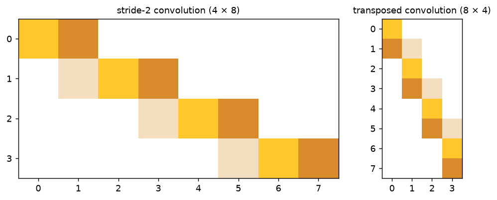
conv_transpose1d with the same kernel and stride. The second is the transpose of the first, to machine precision.
max |M_up - M_down^T| = 0.0e+00
Transposed convolution is not deconvolution
Older papers, and fig. 26 below, call the transposed convolution a “deconvolution”. It does not invert a convolution; it is a learned linear upsampling whose connectivity pattern is the transpose of a strided convolution’s. Prince also notes (p. 181) that transposed convolutions can produce checkerboard artifacts, which is why many modern decoders upsample by interpolation and then apply an ordinary convolution.
6.3 Changing the number of channels
Prince §10.4.3, p. 174; figure on p. 175.
Sometimes we need to change the channel count without pooling, typically so a representation can be added to another branch of the network (the residual connections of Chapter 11). A convolution with kernel size one does this: each output is a weighted sum of all channels at the same position (fig. 21), repeated with different weights for each of the \(C_o\) output channels, so the weights have size \(1 \times 1 \times C_i \times C_o\). With a bias and activation, a 1×1 convolution is the same fully connected network run on the channel vector at every position. The cell confirms it.
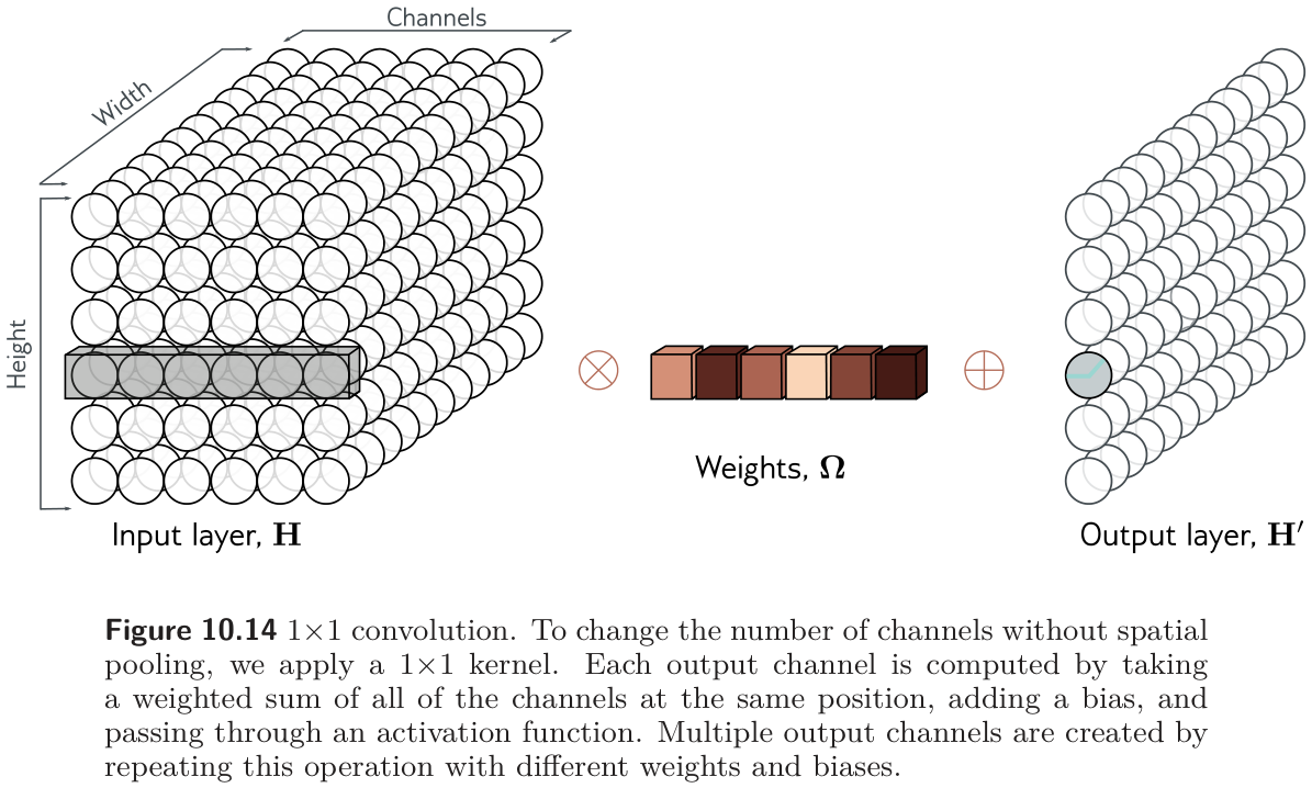
1x1 convolution == per-position fully connected layer: True (parameters: 45 vs 45)7 Applications
Prince §10.5, pp. 174–179.
Prince closes the chapter with three computer-vision tasks, which also serve as a short history of the field.
7.1 Image classification
Prince §10.5.1, pp. 174–176; figures on pp. 175–177.
The pioneering work targeted ImageNet (fig. 22): 1,281,167 training images, 50,000 validation and 100,000 test images, each labeled with one of 1,000 categories. The standard input is a 224×224 RGB image, and the output a distribution over the 1,000 classes. In 2011, before deep networks, the best method had about 25% top-5 error (the correct class is not among the five most probable). Five years later, the best deep networks beat human performance.
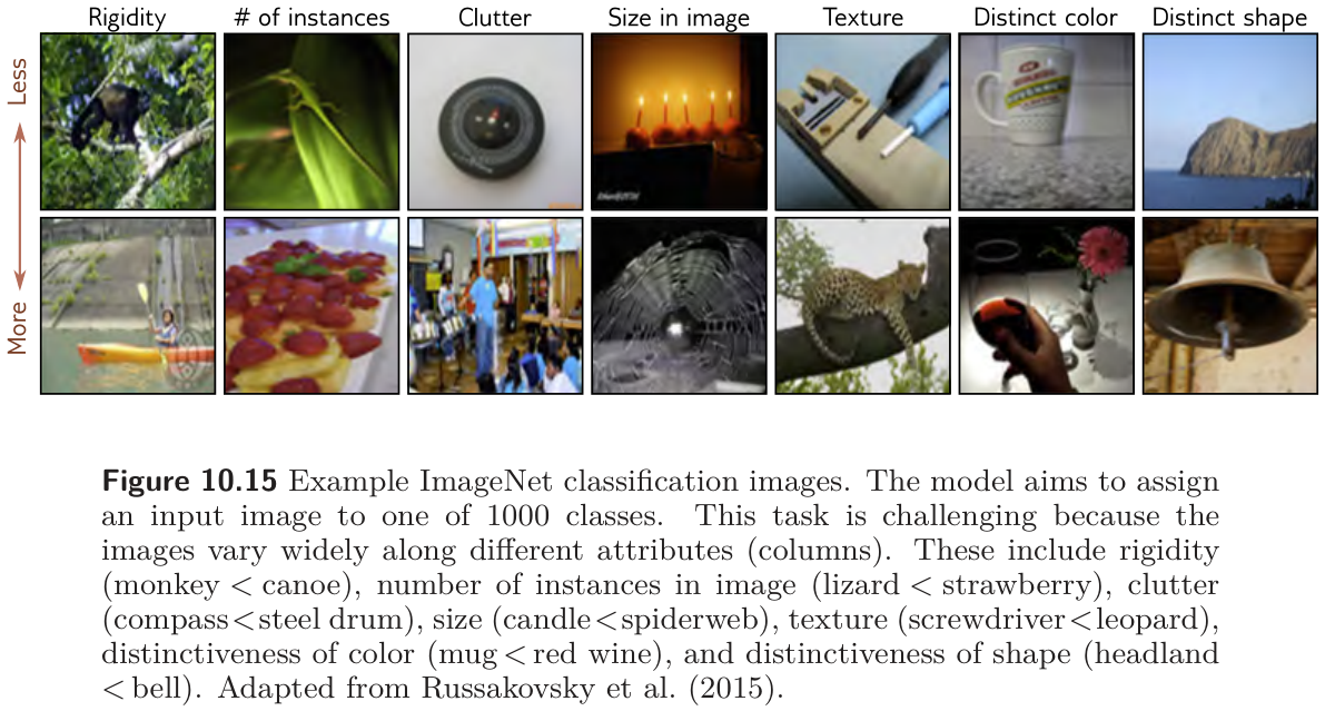
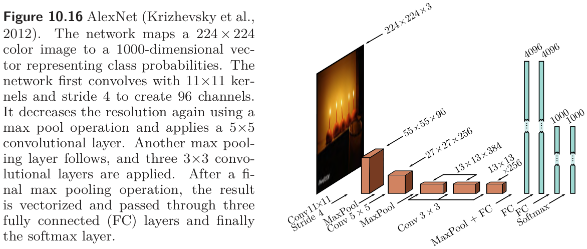
AlexNet (2012, fig. 23) was the first convolutional network to do well on this task (Krizhevsky, Sutskever, and Hinton 2012). It has eight hidden layers with ReLU activations: five convolutional and three fully connected. It begins by downsampling with an 11×11 kernel at stride four to make 96 channels, max pools, applies a 5×5 convolution to make 256 channels, max pools again, applies three 3×3 convolutions, and ends at a 13×13 representation with 256 channels that is flattened into a vector of length 43,264 and passed through fully connected layers of 4,096, 4,096, and 1,000 units, then a softmax. It has about 60 million parameters, most of them in the fully connected layers at the end. Training used every Week 9 trick available at the time: the dataset was augmented by a factor of 2,048 with spatial transformations and intensity changes, five cropped and mirrored versions of each test image were averaged, dropout was applied in the fully connected layers, and an L2 penalty was used. It reached 16.4% top-5 and 38.1% top-1 error, a result Prince credits with kick-starting the modern era of AI research.
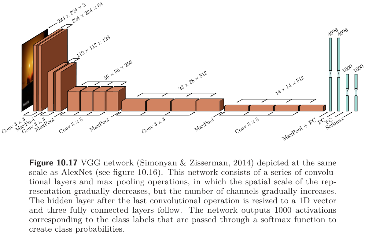
VGG (fig. 24) reached 6.8% top-5 and 23.7% top-1 error (Simonyan and Zisserman 2015). Structurally it is the same recipe — convolutions interspersed with max pooling, spatial size falling while the channel count rises, three fully connected layers at the end — and it, too, was trained with augmentation, weight decay, and dropout. The important difference was depth: 19 hidden layers and 144 million parameters. For several years performance on ImageNet improved as networks got deeper, which Prince takes as evidence that depth matters.
The cell walks through torchvision’s implementations of both networks, listing the shape and parameter count of every weighted layer (problems 10.16 and 10.18). Note that torchvision’s AlexNet is the single-GPU variant with 64, 192, 384, 256, and 256 channels rather than the paper’s 96, 256, 384, 384, and 256, so its total differs slightly from the book’s figure.
AlexNet (torchvision variant)
  conv    3 -> 64   kernel 11x11, stride 4                   23,296
  conv   64 -> 192  kernel 5x5, stride 1                    307,392
  conv  192 -> 384  kernel 3x3, stride 1                    663,936
  conv  384 -> 256  kernel 3x3, stride 1                    884,992
  conv  256 -> 256  kernel 3x3, stride 1                    590,080
  fully connected  9,216 -> 4,096                        37,752,832
  fully connected  4,096 -> 4,096                        16,781,312
  fully connected  4,096 -> 1,000                         4,097,000
  convolutional layers  5                                 2,469,696
  fully connected layers  3                                58,631,144
  total                                                               61,100,840

VGG-19
  convolutional layers 16                                20,024,384
  fully connected layers  3                               123,642,856
  total                                                              143,667,240
7.2 Object detection
Prince §10.5.2, p. 177; figure on p. 178.
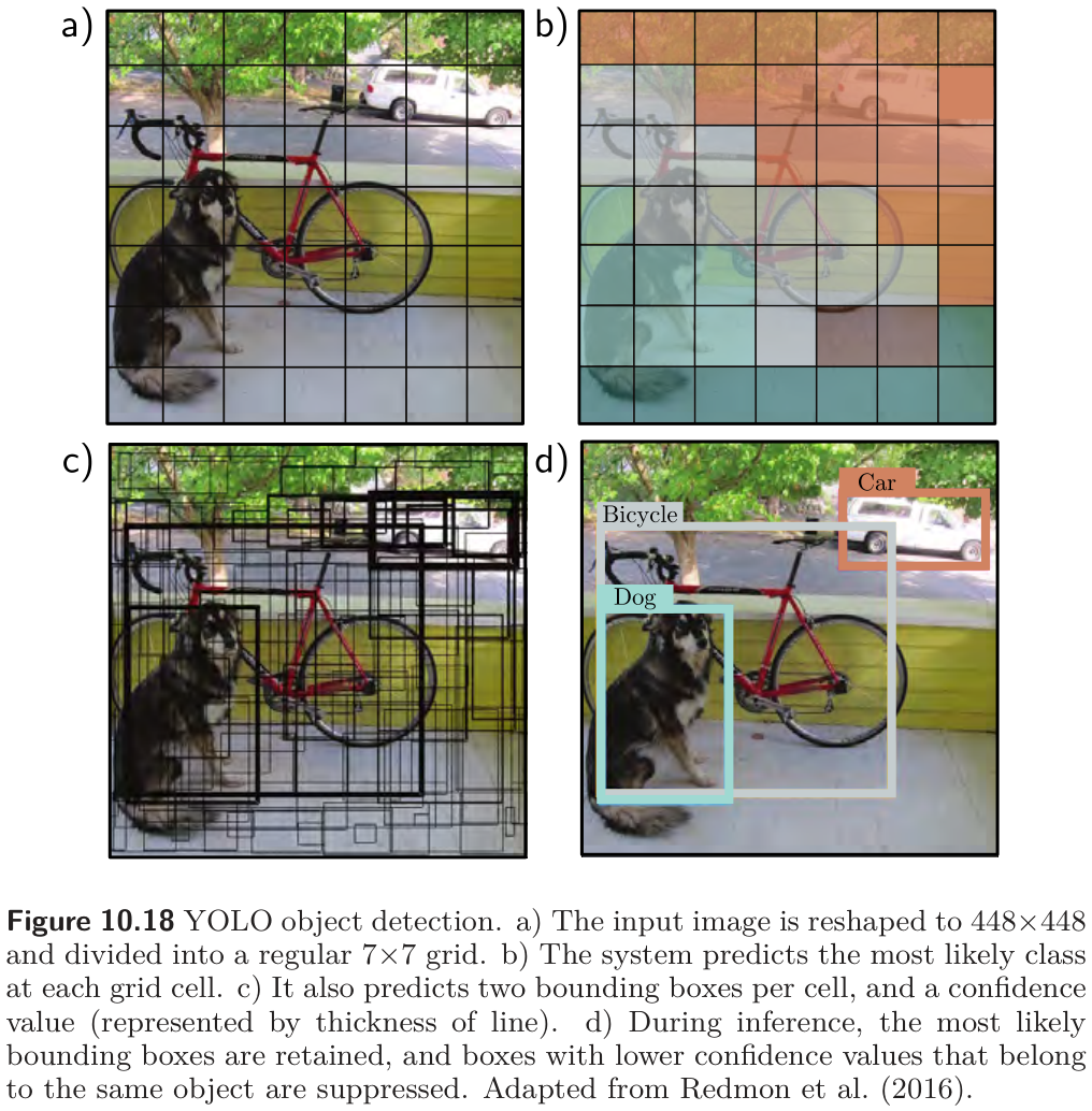
Object detection identifies and localizes multiple objects in an image. YOLO (“You Only Look Once”, fig. 25) (Redmon et al. 2016) passes a 448×448 image through 24 convolutional layers, VGG-style, down to a 7×7 representation with 1,024 channels, then two fully connected layers. The output encodes, for each cell of a 7×7 grid, the most likely class and a fixed number of bounding boxes, each described by five numbers: the \(x\) and \(y\) position of its center, its height and width, and a confidence that estimates the overlap with the true box. The network is trained with momentum, weight decay, dropout, and augmentation, and uses transfer learning: it is first trained to classify ImageNet and then fine-tuned for detection. A heuristic post-processing step removes low-confidence boxes and suppresses duplicate boxes for the same object.
7.3 Semantic segmentation
Prince §10.5.3, pp. 178–179; figures on pp. 179–180.
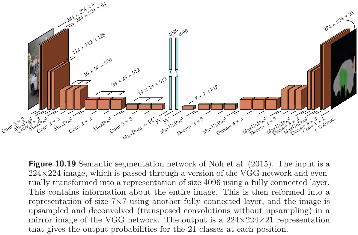
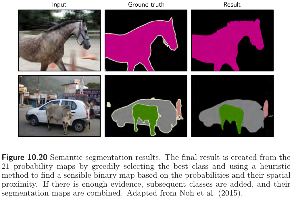
Semantic segmentation assigns a class label to every pixel. The early network of fig. 26 maps a 224×224 image to a 224×224×21 array of class probabilities. Its first half is a smaller VGG (thirteen convolutional layers) that shrinks the representation to 14×14, then 7×7, then two fully connected layers of size 4,096 that no longer have any spatial layout — they integrate information from the whole image. The second half mirrors the first: a fully connected layer reconstitutes a 7×7×512 representation, and a series of max unpooling and transposed convolution layers grows it back to full resolution, ending with a 1×1 convolution to 21 channels and a softmax at every position. The downsampling half is an encoder, the upsampling half a decoder, and the whole an encoder–decoder or hourglass network. The final label map is assembled greedily, class by class, with a heuristic that encourages connected regions (fig. 27).
7.4 Where the field went
Prince §10.6 and chapter notes, pp. 179–184; figure on p. 182.
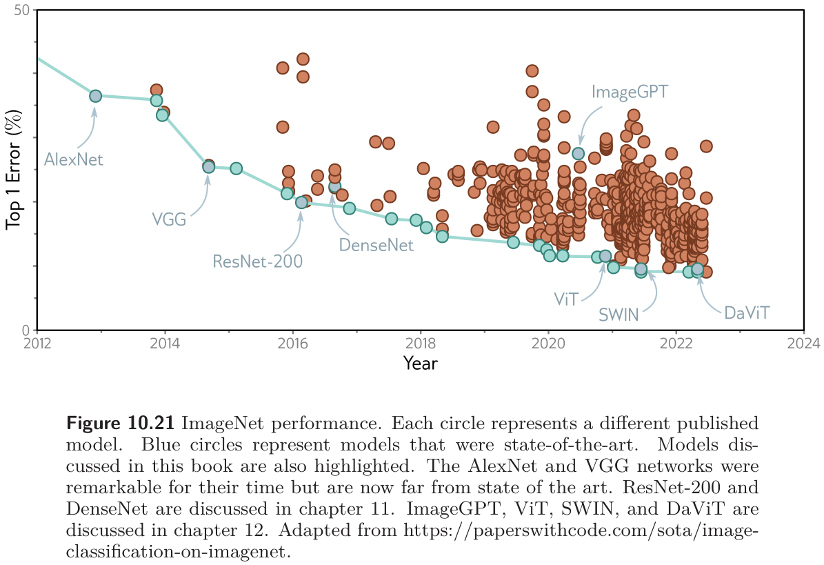
fig. 28 plots ImageNet top-1 error over a decade. AlexNet and VGG were remarkable for their time but are far from the current state of the art. The next two steps on the curve are ResNet and DenseNet — the subject of the second half of this note — and the models after 2020 (ViT, SWIN, DaViT) are transformers, the subject of the next one.
The chapter notes (pp. 180–184) are worth a skim. Two items matter for practice. First, dropout works poorly on convolutional layers, because neighboring pixels carry nearly the same information, so a dropped unit is replaced by its neighbors; spatial dropout (drop whole channels) and cutout (mask a square of the input) are the convolutional substitutes. Second, standard convolutional layers have many cheaper variants — depthwise, grouped, and separable convolutions — that reduce \(C_i C_o K^2\) toward \(C K^2\) and are the basis of mobile architectures.
The recipe, in one paragraph
Every classifier in this section follows the same template, and so does the one you will build at the end of this note. Convolutional layers with small kernels, interspersed with downsampling by a factor of two. As the network deepens, the spatial size halves and the channel count doubles, so the number of values per layer falls slowly while the receptive field grows quickly. At the end, something that integrates over the whole image — fully connected layers in AlexNet and VGG, global average pooling in everything since — and a softmax. If the output is an image, a mirrored decoder upsamples back.
8 Residual Networks
Prince, Chapter 11 opening, p. 186.
Going from AlexNet’s eight layers to VGG’s eighteen improved ImageNet performance, so the obvious next experiment was to add more. It failed: performance decreased when many more layers were added. Chapter 11 explains why, and introduces the two components that fixed it. A residual block computes an additive change to the representation instead of replacing it, which makes very deep networks trainable but causes activations to grow exponentially with depth at initialization. Batch normalization re-centers and rescales the activations at each layer to compensate. Together they allow networks hundreds of layers deep.
8.1 Sequential processing and its limits
Prince §11.1, pp. 186–189; figures on pp. 187–188.
Every network so far processes data sequentially: each layer receives the previous layer’s output and passes its own to the next (fig. 29). For three hidden layers,
\[ \begin{aligned} \mathbf{h}_1 &= \mathbf{f}_1[\mathbf{x}, \boldsymbol{\phi}_1] \\ \mathbf{h}_2 &= \mathbf{f}_2[\mathbf{h}_1, \boldsymbol{\phi}_2] \\ \mathbf{h}_3 &= \mathbf{f}_3[\mathbf{h}_2, \boldsymbol{\phi}_3] \\ \mathbf{y} &= \mathbf{f}_4[\mathbf{h}_3, \boldsymbol{\phi}_4], \end{aligned} \tag{10}\]
or, as one nested function, \(\mathbf{y} = \mathbf{f}_4\big[\mathbf{f}_3\big[\mathbf{f}_2\big[\mathbf{f}_1[\mathbf{x},\boldsymbol{\phi}_1],\boldsymbol{\phi}_2\big],\boldsymbol{\phi}_3\big],\boldsymbol{\phi}_4\big]\). In a fully connected network each \(\mathbf{f}_k\) is a linear transformation followed by an activation; in a convolutional network it is a set of convolutions followed by an activation.

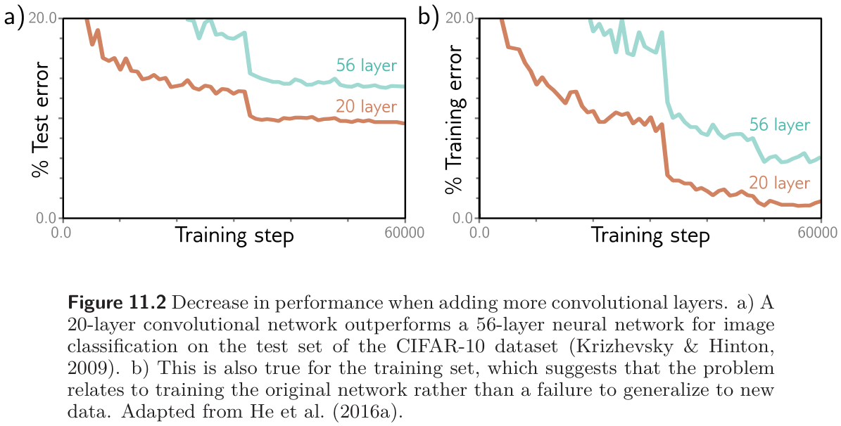
In principle we can stack as many layers as we like. In practice, fig. 30 shows a 56-layer convolutional network doing worse than a 20-layer one on CIFAR-10 — on the test set and on the training set. The training-set result is the diagnostic: this is not a failure to generalize but a failure to train, which is surprising when more capacity usually helps (figure 8.10 in Week 8).
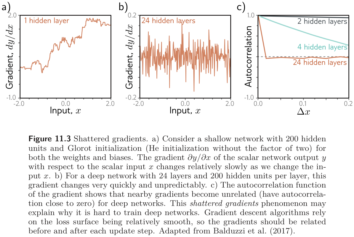
The phenomenon is not fully understood. Prince’s conjecture is about the geometry of the loss surface rather than the size of the gradients. With proper initialization (Week 7) the gradient at the start is reasonable — it neither explodes nor vanishes. But a derivative describes an infinitesimal change, and an optimizer takes a finite step. In a very deep network, any reasonable step may land somewhere whose gradient is unrelated to the one just used: the loss surface looks like a vast field of tiny mountains rather than a smooth valley. fig. 31 shows the supporting evidence from networks with one input and one output. For a shallow network, the gradient \(\partial y / \partial x\) changes slowly with \(x\); for a 24-layer network it changes unpredictably, and the autocorrelation function of the gradient drops to zero over tiny distances. This is the shattered gradients phenomenon (Balduzzi et al. 2017).
The reason is visible in the chain rule. The derivative of the output with respect to the first layer of eq. 10 is
\[ \frac{\partial \mathbf{y}}{\partial \mathbf{f}_1} = \frac{\partial \mathbf{f}_4}{\partial \mathbf{f}_3} \frac{\partial \mathbf{f}_3}{\partial \mathbf{f}_2} \frac{\partial \mathbf{f}_2}{\partial \mathbf{f}_1}, \tag{11}\]
and when the parameters of \(\mathbf{f}_1\) change, every factor in the product changes, because every later layer is computed from \(\mathbf{f}_1\). The gradient at each training example can therefore be completely different after a step.
The cell reproduces the experiment. One remark before the plot: Prince’s own notebook 11.1 reports that a plain deep ReLU network with Glorot initialization does not visibly reproduce fig. 31b — its gradient just shrinks toward zero. The original experiment of Balduzzi et al. used batch normalization in the deep network, which keeps every layer’s signal at unit scale across the input range. We therefore show both the plain and the normalized 24-layer networks, plus a residual network as a preview of the cure.
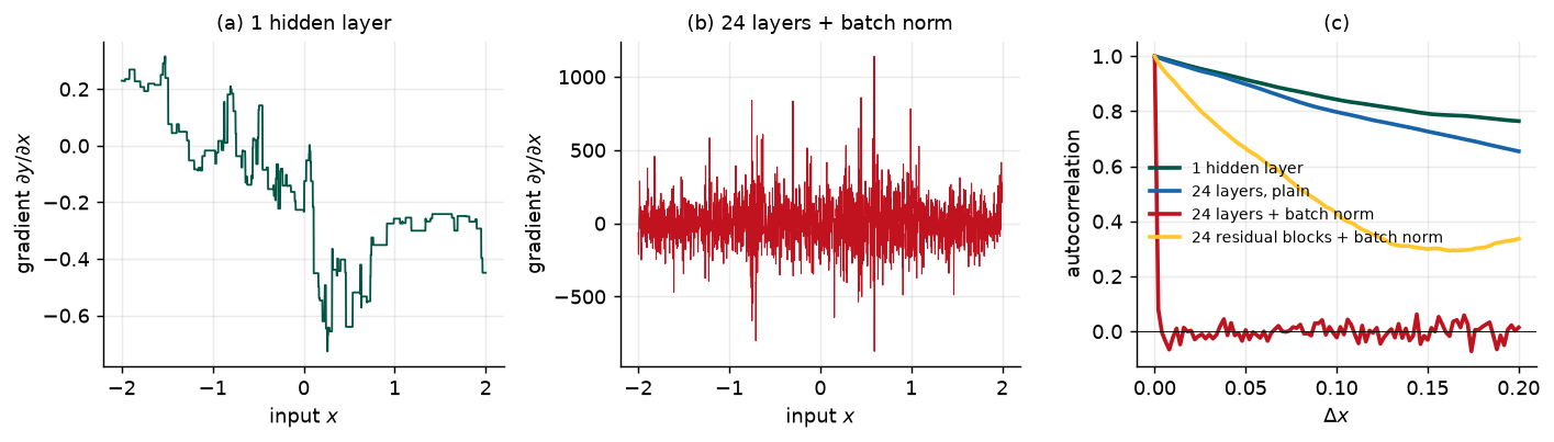
network                               gradient std  autocorrelation at one grid step
1 hidden layer                            2.38e-01                             0.996
24 layers, plain                          2.91e-04                             0.995
24 layers + batch norm                    1.57e+02                             0.079
24 residual blocks + batch norm           1.35e+01                             0.976
8.2 Residual connections and residual blocks
Prince §11.2, pp. 189–192; figures on pp. 190–191.
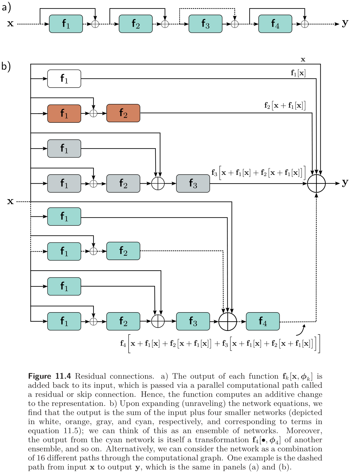
A residual or skip connection is a branch in the computational path that adds each layer’s input back to its output (fig. 33a). The network of eq. 10 becomes
\[ \begin{aligned} \mathbf{h}_1 &= \mathbf{x} + \mathbf{f}_1[\mathbf{x}, \boldsymbol{\phi}_1] \\ \mathbf{h}_2 &= \mathbf{h}_1 + \mathbf{f}_2[\mathbf{h}_1, \boldsymbol{\phi}_2] \\ \mathbf{h}_3 &= \mathbf{h}_2 + \mathbf{f}_3[\mathbf{h}_2, \boldsymbol{\phi}_3] \\ \mathbf{y} &= \mathbf{h}_3 + \mathbf{f}_4[\mathbf{h}_3, \boldsymbol{\phi}_4]. \end{aligned} \tag{12}\]
Each \(\mathbf{f}_k\) now learns an additive change to the current representation, so its output must have the same size as its input. Each sum of input and processed output is a residual block. Substituting each line into the next “unravels” the network:
\[ \begin{aligned} \mathbf{y} = \mathbf{x} &+ \mathbf{f}_1[\mathbf{x}] \\ &+ \mathbf{f}_2\big[\mathbf{x} + \mathbf{f}_1[\mathbf{x}]\big] \\ &+ \mathbf{f}_3\big[\mathbf{x} + \mathbf{f}_1[\mathbf{x}] + \mathbf{f}_2[\mathbf{x} + \mathbf{f}_1[\mathbf{x}]]\big] \\ &+ \mathbf{f}_4\big[\mathbf{x} + \mathbf{f}_1[\mathbf{x}] + \mathbf{f}_2[\cdots] + \mathbf{f}_3[\cdots]\big], \end{aligned} \tag{13}\]
with the parameters omitted. The output is the input plus four smaller networks, one per line (fig. 33b), so one reading is that residual connections turn the network into an ensemble of shallower networks whose outputs are summed. A complementary reading counts paths: the four-block network has \(2^4 = 16\) paths from input to output, of every length from zero (the identity) to four, and \(\mathbf{f}_1\) sits on eight of them.
The derivative with respect to the first layer now has one term per path through \(\mathbf{f}_1\):
\[ \frac{\partial \mathbf{y}}{\partial \mathbf{f}_1} = \mathbf{I} + \frac{\partial \mathbf{f}_2}{\partial \mathbf{f}_1} + \Big(\frac{\partial \mathbf{f}_3}{\partial \mathbf{f}_1} + \frac{\partial \mathbf{f}_3}{\partial \mathbf{f}_2}\frac{\partial \mathbf{f}_2}{\partial \mathbf{f}_1}\Big) + \Big(\frac{\partial \mathbf{f}_4}{\partial \mathbf{f}_1} + \frac{\partial \mathbf{f}_4}{\partial \mathbf{f}_2}\frac{\partial \mathbf{f}_2}{\partial \mathbf{f}_1} + \frac{\partial \mathbf{f}_4}{\partial \mathbf{f}_3}\frac{\partial \mathbf{f}_3}{\partial \mathbf{f}_1} + \frac{\partial \mathbf{f}_4}{\partial \mathbf{f}_3}\frac{\partial \mathbf{f}_3}{\partial \mathbf{f}_2}\frac{\partial \mathbf{f}_2}{\partial \mathbf{f}_1}\Big). \tag{14}\]
Compare eq. 11, which had only the last, longest term. The identity says that a change in \(\boldsymbol{\phi}_1\) reaches the output directly; the short chains are better behaved than the long one; and since every layer’s gradient contains an identity and several short chains, residual networks suffer far less from shattered gradients — which is what the gold curve in fig. 32c showed.
Worked: counting paths (problem 11.2)
Unraveling \(K\) residual blocks gives one path for every subset of the blocks (each block is either on the path or skipped), so there are \(2^K\) paths in all, and the number of paths of length \(\ell\) is the number of \(\ell\)-subsets, \(\binom{K}{\ell}\). For \(K = 4\) that is 1, 4, 6, 4, 1; for \(K = 3\) it is 1, 3, 3, 1; for \(K = 5\) it is 1, 5, 10, 10, 5, 1. The average path length is \(K/2\), which is one way to see why a 200-block ResNet behaves like a combination of 100-block networks rather than one 200-block network.
 blocks K  paths of length 0, 1, ..., K              total
        3  [1, 3, 3, 1]                                  8
        4  [1, 4, 6, 4, 1]                              16
        5  [1, 5, 10, 10, 5, 1]                         32
        8  [1, 8, 28, 56, 70, 56, 28, 8, 1]            256
Order of operations. The additive function \(\mathbf{f}[\bullet]\) must contain a nonlinearity, or the whole network is linear. But if the ReLU comes last, as in an ordinary layer, every block can only add non-negative quantities (fig. 34a). So residual blocks usually apply the activation first and end with the linear transformation or convolution (fig. 34b), possibly with several layers in between (fig. 34c). One consequence: a block that starts with a ReLU does nothing if the network input is entirely negative, so networks start with a plain linear layer rather than a residual block.
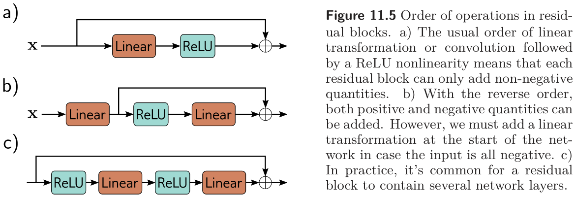
Residual connections roughly double the depth at which a network can be trained before performance degrades. To go further we need to look at what happens to the variance of the activations in the forward pass.
8.3 Exploding activations in residual networks
Prince §11.3, p. 192; figure on p. 193.
Week 7 initialized the parameters so that the variance of the activations stays constant from layer to layer in the forward pass, and the variance of the gradients in the backward pass. He initialization does this for ReLU layers: biases zero, weights normal with variance \(2 / D_h\). In a residual network, vanishing is no longer a concern — every layer has a direct path to the output — but there is a new problem. The two branches of each block, the skip and the processing, carry uncorrelated variability, so when they are added the variances add. He initialization makes the processing branch’s variance equal to its input’s, so the variance doubles at every block (fig. 35a): after \(K\) blocks it is \(2^K\), and the forward pass overflows floating point long before \(K\) reaches a few hundred. The same argument applies to the gradients in the backward pass, so residual networks with He initialization still have exploding gradients.
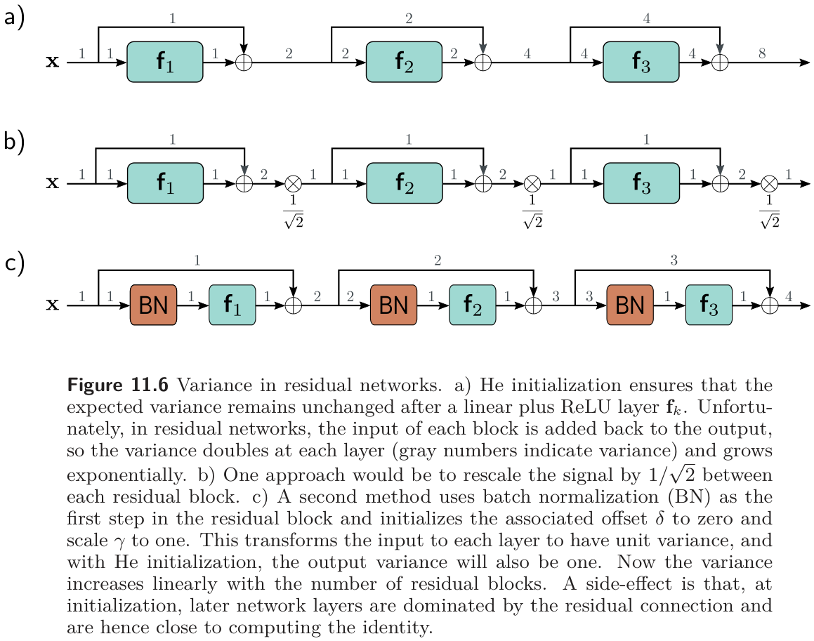
One fix multiplies the output of each block by \(1/\sqrt{2}\) (fig. 35b). The usual fix is batch normalization at the start of each block (fig. 35c), which transforms the block’s input to unit variance so that the processing branch adds exactly one unit of variance: the variance after block \(k\) is \(k + 1\), growing linearly instead of exponentially. The cell measures all three.
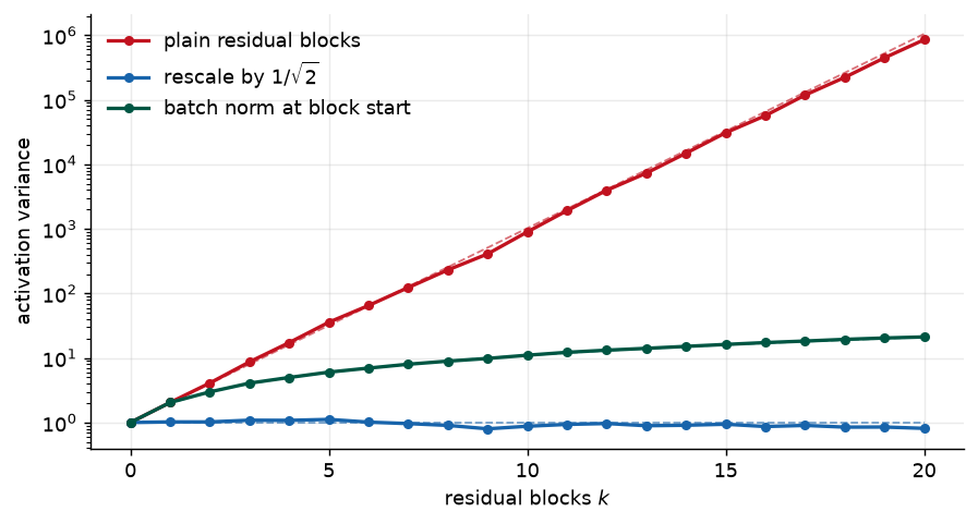
plain      variance after 5, 10, 20 blocks:         35.8        897.4      852,254.4
rescale    variance after 5, 10, 20 blocks:          1.1          0.9            0.8
batchnorm  variance after 5, 10, 20 blocks:          6.0         11.0           21.2
8.4 Batch normalization
Prince §11.4, pp. 192–195.
Batch normalization (BatchNorm) shifts and rescales each activation \(h\) so that its mean and variance across the current batch \(\mathcal{B}\) become values that are learned. First compute the empirical mean and standard deviation of that activation over the batch,
\[ m_h = \frac{1}{|\mathcal{B}|} \sum_{i \in \mathcal{B}} h_i, \qquad s_h = \sqrt{\frac{1}{|\mathcal{B}|} \sum_{i \in \mathcal{B}} (h_i - m_h)^2}, \tag{15}\]
then standardize,
\[ h_i \leftarrow \frac{h_i - m_h}{s_h + \epsilon} \qquad \forall i \in \mathcal{B}, \tag{16}\]
where \(\epsilon\) prevents division by zero if every member of the batch has the same value, and finally scale by \(\gamma\) and shift by \(\delta\),
\[ h_i \leftarrow \gamma\, h_i + \delta \qquad \forall i \in \mathcal{B}. \tag{17}\]
After this the activation has mean \(\delta\) and standard deviation \(\gamma\) across the batch, and both are learned. Every hidden unit has its own \(\gamma\) and \(\delta\): a fully connected network with \(K\) layers of \(D\) units has \(KD\) of each. In a convolutional network the statistics are computed over the batch and the spatial positions, and there is one \(\gamma, \delta\) pair per channel, so \(K\) layers of \(C\) channels have \(KC\) of each. At test time there is no batch, so the statistics \(m_h\) and \(s_h\) are computed over the whole training set (in practice, as running averages during training) and frozen into the network. In PyTorch, model.train() and model.eval() switch between the two behaviors, which is why forgetting eval() at test time is a classic bug.
hand-coded BatchNorm matches nn.BatchNorm1d:          True
output unchanged when the incoming weights double:    True
output mean and sd per unit after BatchNorm:          [0.0, -0.0, -0.0, 0.0]  [1.0, 1.0, 1.0, 1.0]

problem 11.6: parameters without BatchNorm 3,841, with BatchNorm 4,241 (+ 400 = 2 x 20 units x 10 layers)
Costs and benefits (§11.4.1, p. 194). The second line of the printout is the cost. BatchNorm makes the network invariant to rescaling the weights and biases feeding each unit — double them and the standardization undoes it — so a large family of parameter settings now produces the same function, and the layer adds two new parameters per unit to compensate for that redundancy. That is inefficient, but three benefits outweigh it.
- Stable forward propagation. With \(\delta = 0\) and \(\gamma = 1\) at initialization, every output activation has unit variance. In a residual network the variance still grows, but linearly (fig. 36). A side effect: at initialization later blocks change the representation proportionally less than earlier ones, so the network is effectively shallower at the start of training and can grow its own depth by increasing \(\gamma\) in later layers.
- Higher learning rates. Theory and experiment agree that BatchNorm makes the loss surface and its gradient change more smoothly — it reduces shattering — so larger steps are safe, and Week 9 showed that larger learning rates generalize better.
- Regularization. The normalization of each example depends on which other examples share its batch, so it is slightly different at every iteration. That is injected noise, which Chapter 9 listed among the regularizers.
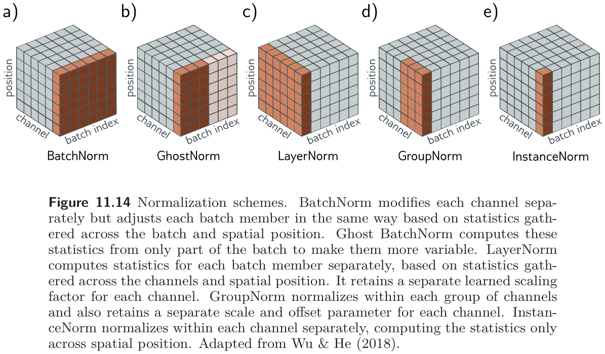
The chapter notes (pp. 203–204) add that BatchNorm’s original rationale, reducing internal covariate shift, has not held up (Santurkar et al. 2018); the smoothing of the loss surface is the better-supported explanation. They also survey the alternatives of fig. 37: LayerNorm normalizes each example over its own channels and positions and needs no batch (it is the normalization in transformers, next week); GroupNorm and InstanceNorm normalize over subsets of channels. All keep a learned \(\gamma\) and \(\delta\) per channel.
8.5 Common residual architectures
Prince §11.5, pp. 195–199; figures on pp. 196–200.
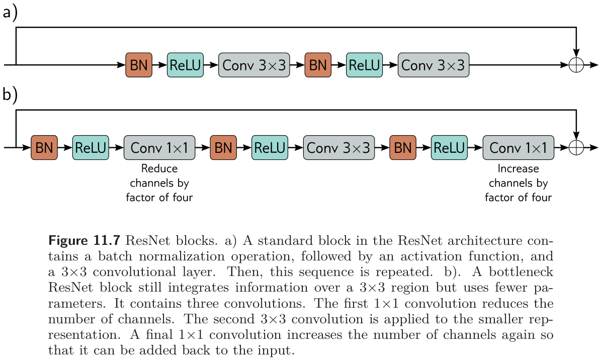
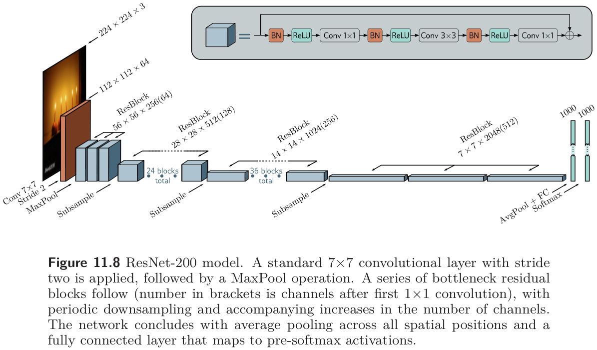
ResNet (§11.5.1) (He et al. 2016a, 2016b). In the standard block a BatchNorm, a ReLU, and a 3×3 convolution are applied twice before the result is added back to the input (fig. 38a). For very deep networks the bottleneck block (fig. 38b) saves parameters with three convolutions: a 1×1 that reduces the channel count by a factor of four, a 3×3 on the smaller representation, and a 1×1 that restores the channel count so the result can be added back. Information is still integrated over a 3×3 region, at a fraction of the cost. ResNet-200 (fig. 39) opens with a 7×7 convolution and a max pool, then stacks bottleneck blocks with periodic stride-two downsampling and channel doubling (with zero-channel padding or a 1×1 convolution to match sizes across the change), then global average pooling and a fully connected layer to 1,000 classes. It reached 4.8% top-5 and 20.1% top-1 error, against 16.4%/38.1% for AlexNet and 6.8%/23.7% for VGG, and was among the first networks to exceed the estimated human top-5 error of 5.1%.
problem 11.8, blocks with 512 input and output channels
  standard block   (3x3, 3x3)         4,721,664 parameters
  bottleneck block (1x1, 3x3, 1x1)      280,832 parameters   (16.8x fewer)
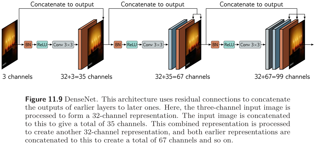
DenseNet (§11.5.2) (Huang et al. 2017). Instead of adding the processed signal to the input, concatenate them along the channel dimension (fig. 40). Each layer then receives the outputs of all previous layers, and an optional 1×1 convolution can map the concatenation back to a smaller size — which lets the network learn to add, to take a weighted sum, or to combine representations in any other way. The channel count grows quickly, so 1×1 bottlenecks are inserted, and the concatenation chain restarts at each downsampling (concatenating representations of different sizes makes no sense). DenseNet matches or beats ResNet at a comparable parameter count, presumably because it reuses earlier processing more flexibly.
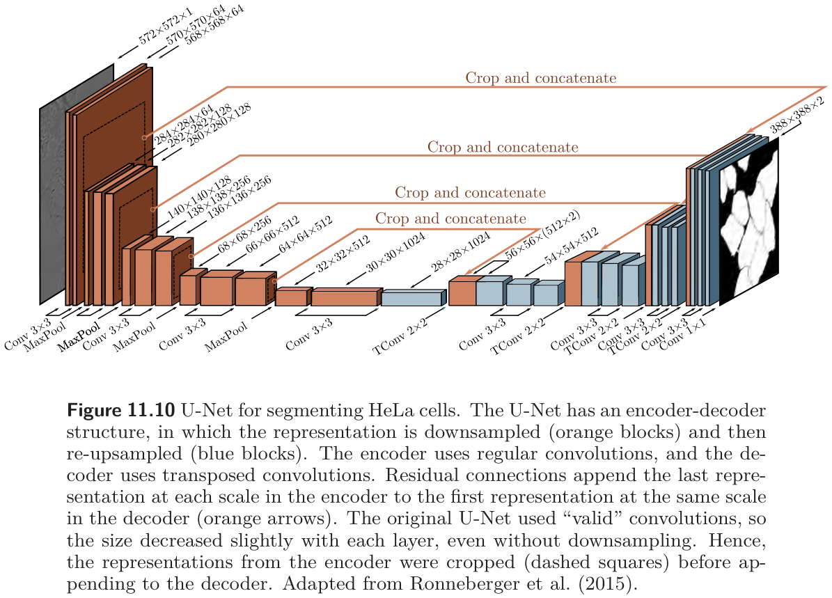
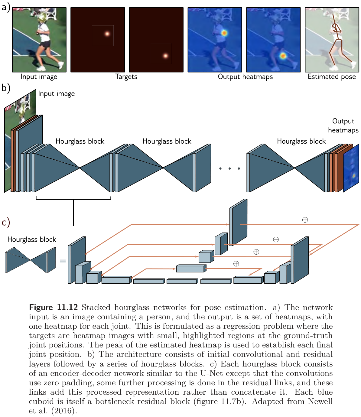
U-Net and hourglass networks (§11.5.3) (Ronneberger, Fischer, and Brox 2015). The encoder–decoder of fig. 26 has a weakness: the low-resolution representation in the middle must remember every high-resolution detail the decoder will need. Residual connections remove that burden by passing each scale’s last encoder representation to the decoder’s first representation at the same scale (fig. 41). The U-Net concatenates them, as DenseNet does. The original used valid convolutions, so each 3×3 layer lost two pixels and the encoder representations had to be cropped before concatenation; later versions zero-pad. Because it is entirely convolutional, a trained U-Net runs on an image of any size. Hourglass networks add further convolutions along the skip connections and add the result rather than concatenating; stacked hourglasses alternate between local and global views and are used for pose estimation, predicting one heat map per joint (fig. 42).
U-Nets in this course
U-Net is the single most reused architecture in applied deep learning: medical segmentation, defect segmentation on production images, depth estimation, inpainting, and image-to-image translation all use it. It also returns in Week 15 as the denoiser inside diffusion models.
8.6 Why do residual networks work so well?
Prince §11.6, p. 199; figure on p. 201.
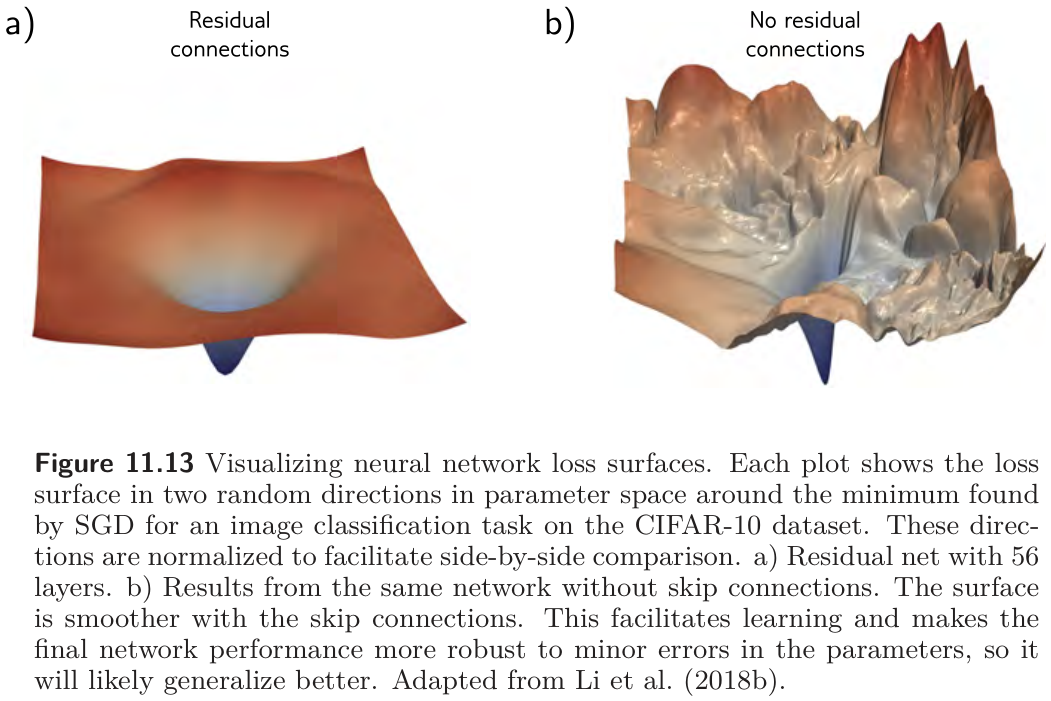
ResNets can be extended to 1,000 layers and still train, and the improvement in classification was first credited to that depth. Two findings complicate the story. Shallower, wider residual networks sometimes beat deeper, narrower ones with the same parameter count (Zagoruyko and Komodakis 2016), and gradients do not propagate effectively along the very long paths of the unraveled network: Veit et al. (Veit, Wilber, and Belongie 2016) found that in a 54-block ResNet, almost all gradient came from paths 5 to 17 blocks long, which are 0.45% of the paths, and that deleting individual blocks from a trained ResNet barely hurts it, whereas deleting a layer from VGG is catastrophic. A very deep residual network behaves more like a combination of shallow networks. The current view is that residual connections add value of their own, beyond enabling depth: the loss surface around a minimum is smoother and more predictable with the skip connections than without them (fig. 43), which makes a good, generalizing solution easier to find.
9 Training a CNN in PyTorch
Our own section; the recipe of Prince §10.6 and §11.5.1.
This section shows its code, because the point is the code. The task is a small industrial one: classify 28×28 grayscale patches from an imaginary surface-inspection camera as clean, scratch (a thin bright line at a random position and angle), or pit (a dark blob of random size). The data are synthetic, so you can regenerate as much as you want, and the model is a miniature of the recipe above: three convolution–BatchNorm–ReLU stages, max pooling between the first two, global average pooling, and one linear layer.
def make_defect_images(n, rng, S=28):
    """n patches of size S x S. Class 0: clean; 1: scratch (bright line); 2: pit (dark blob)."""
    yy, xx = np.mgrid[0:S, 0:S]
    X = 0.5 + 0.1 * rng.standard_normal((n, S, S))
    y = rng.integers(0, 3, n)
    for i in range(n):
        if y[i] == 1:
            theta = rng.uniform(0, np.pi)
            cx, cy = rng.uniform(6, S - 6, 2)
            across = np.abs((xx - cx) * np.sin(theta) - (yy - cy) * np.cos(theta))
            along  = np.abs((xx - cx) * np.cos(theta) + (yy - cy) * np.sin(theta))
            X[i][(across < 0.8) & (along < rng.uniform(4, 9))] += 0.3
        elif y[i] == 2:
            cx, cy = rng.uniform(5, S - 5, 2)
            r = rng.uniform(1.2, 2.5)
            X[i] -= 0.35 * np.exp(-((xx - cx) ** 2 + (yy - cy) ** 2) / (2 * r ** 2))
    return torch.tensor(X, dtype=torch.float32).unsqueeze(1), torch.tensor(y)   # (n, 1, S, S)

rng = np.random.default_rng(774)
X_train, Y_train = make_defect_images(3000, rng)
X_test,  Y_test  = make_defect_images(600, rng)
classes = ["clean", "scratch", "pit"]

fig, axes = plt.subplots(1, 8, figsize=(10, 1.7))
for ax, i in zip(axes, range(8)):
    ax.imshow(X_train[i, 0], cmap="gray", vmin=0, vmax=1)
    ax.set_title(classes[Y_train[i]], fontsize=9); ax.set_xticks([]); ax.set_yticks([]); ax.grid(False)
plt.tight_layout()
plt.show()
class DefectNet(nn.Module):
    def __init__(self, n_classes=3):
        super().__init__()
        self.features = nn.Sequential(
            nn.Conv2d(1, 16, 3, padding=1),  nn.BatchNorm2d(16), nn.ReLU(), nn.MaxPool2d(2),   # 28x28 -> 14x14
            nn.Conv2d(16, 32, 3, padding=1), nn.BatchNorm2d(32), nn.ReLU(), nn.MaxPool2d(2),   # 14x14 -> 7x7
            nn.Conv2d(32, 64, 3, padding=1), nn.BatchNorm2d(64), nn.ReLU(),
            nn.AdaptiveAvgPool2d(1), nn.Flatten())                                             # 7x7x64 -> 64
        self.classifier = nn.Linear(64, n_classes)

    def forward(self, x):
        return self.classifier(self.features(x))

torch.manual_seed(774)
net = DefectNet()
print(f"DefectNet: {n_params(net):,} parameters\n")

# Trace the shape of one batch through the network, layer by layer.
h = X_train[:2]
print(f"{'layer':20s}{'output shape (batch, channels, height, width)':>50s}")
print(f"{'input':20s}{str(tuple(h.shape)):>50s}")
for layer in net.features:
    h = layer(h)
    if isinstance(layer, (nn.Conv2d, nn.MaxPool2d, nn.AdaptiveAvgPool2d, nn.Flatten)):
        print(f"{type(layer).__name__:20s}{str(tuple(h.shape)):>50s}")
print(f"{'Linear':20s}{str(tuple(net.classifier(h).shape)):>50s}")
DefectNet: 23,715 parameters
layer output shape (batch, channels, height, width)
input (2, 1, 28, 28)
Conv2d (2, 16, 28, 28)
MaxPool2d (2, 16, 14, 14)
Conv2d (2, 32, 14, 14)
MaxPool2d (2, 32, 7, 7)
Conv2d (2, 64, 7, 7)
AdaptiveAvgPool2d (2, 64, 1, 1)
Flatten (2, 64)
Linear (2, 3)opt = torch.optim.Adam(net.parameters(), lr=1e-3)
g = torch.Generator().manual_seed(774)
def accuracy(model, X, Y):
model.eval() # use the frozen BatchNorm statistics
with torch.no_grad():
return 100 * (model(X).argmax(1) == Y).float().mean().item()
print(f"{'epoch':>5s}{'train loss':>12s}{'train acc':>11s}{'test acc':>10s}")
for epoch in range(1, 7):
net.train() # BatchNorm uses batch statistics
perm, total = torch.randperm(len(X_train), generator=g), 0.0
for i in range(0, len(X_train), 64):
idx = perm[i:i + 64]
loss = F.cross_entropy(net(X_train[idx]), Y_train[idx])
opt.zero_grad(); loss.backward(); opt.step()
total += loss.item() * len(idx)
print(f"{epoch:>5d}{total / len(X_train):>12.3f}{accuracy(net, X_train, Y_train):>10.1f}%{accuracy(net, X_test, Y_test):>9.1f}%")
# Confusion matrix on the test set, and a translation test: shift every test patch by a few pixels.
net.eval()
with torch.no_grad():
pred = net(X_test).argmax(1)
shifted_acc = 100 * (net(torch.roll(X_test, shifts=(3, -2), dims=(2, 3))).argmax(1) == Y_test).float().mean().item()
print(f"\n{'true \\ predicted':18s}" + "".join(f"{c:>9s}" for c in classes))
for t, name in enumerate(classes):
print(f"{name:18s}" + "".join(f"{int(((Y_test == t) & (pred == p)).sum()):>9d}" for p in range(3)))
print(f"\ntest accuracy after shifting every patch by (3, -2) pixels: {shifted_acc:.1f}%")epoch train loss train acc test acc
1 0.549 60.8% 61.7%
2 0.225 95.9% 95.0%
3 0.120 98.4% 98.5%
4 0.076 98.8% 98.3%
5 0.055 99.0% 98.3%
6 0.039 99.5% 99.0%
true \ predicted clean scratch pit
clean 219 0 0
scratch 3 187 0
pit 3 0 188
test accuracy after shifting every patch by (3, -2) pixels: 96.8%Three things to notice. The shape trace shows the recipe: spatial size 28 → 14 → 7 → 1 while channels go 1 → 16 → 32 → 64, and global average pooling means the classifier never sees a position, which is where the translation invariance of the last line comes from: shifting every test patch by a few pixels costs only a couple of points of accuracy. The whole network has about 24,000 parameters, fewer than half of the fully connected MNIST-1D network that worked on a 40-sample input, and it would have the same count on 280×280 patches. And net.train() / net.eval() matters: BatchNorm normalizes by batch statistics in one mode and by the frozen training-set statistics in the other, and evaluating in training mode on a small batch gives noisy, sometimes wrong, predictions.
10 Summary
Convolutional layers compute each hidden unit as a weighted sum of nearby inputs, plus a bias, through an activation function, with the same weights and bias at every position. They have far fewer parameters than fully connected layers, a count that does not grow with the image size, and they are equivariant to translation, which is the right inductive bias for images — the MNIST-1D experiment showed a 2,050-parameter convolutional network beating a 59,065-parameter fully connected one that could have imitated it. Several kernels in parallel give channels; stacked layers grow receptive fields; stride and pooling halve the spatial size while channels double; a 1×1 convolution changes the channel count; transposed convolutions and unpooling scale back up when the output is an image. AlexNet, VGG, YOLO, and the encoder–decoder segmentation network are all this recipe at different depths.
Depth helps, up to a point: beyond it, a sequential network becomes hard to train, plausibly because its gradients shatter. A residual block adds its input back to its output, which gives every layer a direct path to the loss and turns the network into an ensemble of shallow paths, at the price of activations whose variance doubles at every block. Batch normalization standardizes each unit over the batch and then applies a learned scale and shift, making the growth linear, smoothing the loss surface enough for larger learning rates, and adding a little regularizing noise. ResNet, its bottleneck block, DenseNet’s concatenation, and U-Net’s skip connections across an encoder–decoder are the standard ways of putting these pieces together.
Next: Chapter 12 replaces the convolution’s fixed, local weighted sum with self-attention, a weighted sum whose weights are computed from the data itself — the transformer, which now also holds the ImageNet records in fig. 28.
11 Exercises
1. (UDL 10.2, 10.3, 10.4) Write the equation, in the style of eq. 3, for a 1D convolution with (a) kernel size three and stride two (fig. 4a–b); (b) kernel size three and dilation rate two (fig. 4d); (c) kernel size seven, dilation rate three, and stride three. For (c), use eq. 4 to find how many outputs a 40-dimensional input produces, and check against the shape-calculator cell.
2. (UDL 10.8 and 10.14) A 1D network’s input has three channels. The first hidden layer uses kernel size three and has four channels; the second uses kernel size five and has ten channels. How many weights and biases does each layer need? Then do the same for a 2D layer with a 5×5 kernel, three input channels, and ten output channels. Confirm with the parameter-count cell.
3. (UDL 10.9, 10.10, 10.11) Compute the receptive field at the third layer of (a) three zero-padded layers of kernel size three and stride one; (b) the same with kernel size seven; (c) a layer with kernel size five and stride two, then kernel size three, then kernel size five with dilation two. Use eq. 8, then verify (a) and (c) against fig. 9.
4. (UDL 10.12 and 10.16*) (a) The network of fig. 10 was trained with batch size 100 on 4,000 examples for 100,000 steps. How many epochs is that? (b) For AlexNet as drawn in fig. 23 (channels 96, 256, 384, 384, 256; fully connected 4,096, 4,096, 1,000; a 13×13×256 representation before the first fully connected layer), compute the parameters of every layer and the total. Compare with the torchvision variant in the architecture-table cell and explain the difference.
5. (UDL 10.15) Draw the 1D weight matrix that keeps every other input (the 1D version of fig. 16a). Show that the matrix for a convolution with kernel size three and stride two (fig. 6b) is the product of this sampling matrix and the stride-one matrix (fig. 6a). What does this say about what a strided convolution computes and does not compute?
6. The MNIST-1D experiment (fig. 12) shows the fully connected network reaching lower training error sooner and higher test error. Explain both halves using (a) the “smaller family of plausible functions” reading and (b) the “infinite penalty” reading of §10.2.7. Then say which of the four mechanisms in figure 9.14 (Week 9) the convolutional structure belongs to.
7. (UDL 11.2 and 11.4*) (a) How many paths of each length are there in a residual network with three blocks? With five? State the rule for \(K\) blocks and check the path-count cell. (b) Explain why the two branches of a residual block are uncorrelated at initialization, and show that the variance of a sum of uncorrelated variables is the sum of their variances. Use this to derive the dashed curves in fig. 36.
8. (UDL 11.6 and 11.8) (a) A fully connected network has one input, one output, and ten hidden layers of twenty units. Count its parameters, then count them again with BatchNorm between each linear transformation and ReLU. (b) Count the parameters of the standard and bottleneck residual blocks of fig. 38 with 512 input and output channels (the bottleneck reduces to 128). Both answers are printed on this page; show the arithmetic.
9. (UDL 11.7*) An L2 penalty is applied to the convolutional weights in the block of fig. 38a but not to the \(\gamma\) parameters of the BatchNorm layers that follow them. What do you expect to happen to the weights and to \(\gamma\) as training proceeds, and why does the network’s function not change? Which line of the batchnorm-check cell is the relevant evidence?
10. (UDL 11.9) A U-Net is fully convolutional and can be run on an image of any size after training. Why do we nevertheless not train it on a collection of arbitrarily sized images? (Think about batches and about BatchNorm.)
11. Choosing an architecture. A line produces 2,000 extruded aluminum profiles per hour, photographed at 1,024×256 pixels. You must (a) flag profiles with a surface defect, (b) outline each defect so an operator can see it, and (c) run on an embedded GPU with little memory. For each of (a) and (b), say whether the output should be translation-invariant or equivariant, which architecture family on this page fits, and where downsampling and upsampling occur. For (c), name two ways to cut the parameter count without reducing depth.
12. Computational. Extend the fig-receptive-field cell to 2D: build a stack of nn.Conv2d layers matching the first three layers of AlexNet (11×11 stride 4; 3×3 max pool stride 2; 5×5), differentiate one central output unit with respect to the input, and report the receptive field in pixels (problem 10.17). Then replace the 11×11 layer by three 3×3 layers of stride one and compare receptive field and parameter count.
13. Computational. In the fig-mnist1d-conv-vs-fc cell, (a) replace the three stride-two convolutions by stride-one convolutions with 2×1 max pooling and compare test error; (b) remove the random placement in make_mnist1d so that every template starts at position 10, retrain both networks, and explain what happens to the gap between them; (c) add nn.BatchNorm1d(15) after each convolution and report the change in the number of steps to reach 5% training error.
14. Computational. Turn DefectNet into a residual network: wrap the second and third stages as pre-activation residual blocks (BatchNorm → ReLU → Conv, twice, plus the skip; use a 1×1 convolution on the skip where the channel count changes), and stack eight such blocks. (a) Train it with and without the BatchNorm layers inside the blocks and compare training loss after one epoch. (b) Measure the standard deviation of the activations after each block at initialization, as in fig. 36, in both versions.
12 Textbook Reference Map
Every part of this page, mapped to Prince, Understanding Deep Learning (MIT Press, 2024) (Prince 2024). Page numbers are those of the printed book.
| This page | Prince section | Pages | Figures used |
|---|---|---|---|
| Why Images Need Their Own Layers | Ch. 10 opening | 161 | — |
| Invariance and Equivariance | §10.1 | 161–162 | 10.1 (p. 162) |
| Convolutional Networks for 1D Inputs | §10.2 | 163 | — |
| — The 1D convolution operation | §10.2.1 | 163 | 10.2 (p. 163) |
| — Padding | §10.2.2 | 164 | — |
| — Stride, kernel size, and dilation | §10.2.3 | 164–165 | 10.3 (p. 164) |
| — Convolutional layers | §10.2.4 | 165 | 10.4 (p. 166) |
| — Channels | §10.2.5 | 165–167 | 10.5 (p. 166) |
| — Receptive fields | §10.2.6 | 167 | 10.6 (p. 168) |
| — Example: MNIST-1D | §10.2.7 | 167–170 | 10.7, 10.8 (p. 169) |
| Convolutional Networks for 2D Inputs | §10.3 | 170–171 | 10.9 (p. 171), 10.10 (p. 172) |
| Downsampling and Upsampling | §10.4 | 171 | — |
| — Downsampling | §10.4.1 | 171–172 | 10.11 (p. 173) |
| — Upsampling | §10.4.2; notes | 172–174, 181 | 10.12, 10.13 (p. 173) |
| — Changing the number of channels | §10.4.3 | 174 | 10.14 (p. 175) |
| Applications | §10.5 | 174 | — |
| — Image classification | §10.5.1 | 174–176 | 10.15 (p. 175), 10.16 (p. 176), 10.17 (p. 177) |
| — Object detection | §10.5.2 | 177 | 10.18 (p. 178) |
| — Semantic segmentation | §10.5.3 | 178–179 | 10.19 (p. 179), 10.20 (p. 180) |
| — Where the field went | §10.6; notes | 179–184 | 10.21 (p. 182) |
| Residual Networks | Ch. 11 opening | 186 | — |
| — Sequential processing and its limits | §11.1, §11.1.1 | 186–189 | 11.1 (p. 187), 11.2, 11.3 (p. 188) |
| — Residual connections and residual blocks | §11.2, §11.2.1, §11.2.2 | 189–192 | 11.4 (p. 190), 11.5 (p. 191) |
| — Exploding activations | §11.3 | 192 | 11.6 (p. 193) |
| — Batch normalization | §11.4, §11.4.1; notes | 192–195, 203–204 | 11.14 (p. 204) |
| — Common residual architectures | §11.5.1–§11.5.3 | 195–199 | 11.7, 11.8 (p. 196), 11.9 (p. 197), 11.10 (p. 198), 11.12 (p. 200) |
| — Why residual networks work so well | §11.6; notes | 199, 202 | 11.13 (p. 201) |
| Training a CNN in PyTorch | §10.6, §11.5.1 (recipe) | 179–180, 195 | — |
| Summary | §10.6, §11.7 | 179–180, 199–201 | — |
| Exercises 1–10 | Problems 10.2–10.4, 10.8–10.16, 11.2, 11.4, 11.6–11.9 | 184–185, 205–206 | — |
Equations on this page correspond to Prince as follows: eq. 1 is his (10.1), eq. 2 is (10.2), eq. 3 is (10.3), eq. 5 is (10.4), eq. 6 is (10.5), eq. 9 is (10.6), eq. 10 is (11.1), eq. 11 is (11.3), eq. 12 is (11.4), eq. 13 is (11.5), eq. 14 is (11.6), eq. 15 is (11.7), eq. 16 is (11.8), and eq. 17 is (11.9). Equations eq. 4, eq. 7, and eq. 8 are ours; the first and third are standard results summarized in Dumoulin & Visin’s guide (Dumoulin and Visin 2016).
Figure credits
Figures 10.1–10.21, 11.1–11.10, and 11.12–11.14 are reproduced unaltered from Prince, Understanding Deep Learning (MIT Press, 2024), which is distributed under a Creative Commons CC-BY-NC-ND license, and are used here for non-commercial classroom instruction. Original sources credited within the figures: panels c–f of figure 10.1 are adapted from Bousselham et al. (2021); figure 10.15 from Russakovsky et al. (2015); figure 10.16 depicts AlexNet, Krizhevsky et al. (2012); figure 10.17 depicts VGG, Simonyan & Zisserman (2014); figure 10.18 is adapted from Redmon et al. (2016); figures 10.19 and 10.20 from Noh et al. (2015); figure 10.21 from paperswithcode.com; figure 11.2 from He et al. (2016a); figure 11.3 from Balduzzi et al. (2017); figure 11.10 from Ronneberger et al. (2015); figure 11.12 from Newell et al. (2016); figure 11.13 from Li et al. (2018b); and figure 11.14 from Wu & He (2018). All other figures on this page are generated by the code in this week’s notebook.
13 Further Reading
- Prince, Understanding Deep Learning, Chapters 10 and 11 (Prince 2024) — the assigned reading. The Chapter 10 notes (pp. 180–184) survey convolution variants, pooling, equivariance to other transformations, and detection and segmentation; the Chapter 11 notes (pp. 201–205) cover why residual connections help, the many normalization schemes, and the alternatives to BatchNorm.
- ▶ UDL notebooks 10.1–10.5 and 11.1–11.3 — Prince’s own Colab notebooks for these chapters; links to each are at the top of this page.
- ▶ This week’s notebook — every cell above, in one Colab file.
- Dumoulin & Visin (2016) (Dumoulin and Visin 2016) — A guide to convolution arithmetic for deep learning: every padding, stride, dilation, and transposed-convolution case with animations; the source of eq. 4.
- LeCun et al. (1998) (LeCun et al. 1998) — LeNet, the recognizable ancestor of every network on this page; Krizhevsky, Sutskever & Hinton (2012) (Krizhevsky, Sutskever, and Hinton 2012) — AlexNet; Simonyan & Zisserman (2015) (Simonyan and Zisserman 2015) — VGG.
- Redmon et al. (2016) (Redmon et al. 2016) — YOLO; Noh, Hong & Han (2015) (Noh, Hong, and Han 2015) — the deconvolution segmentation network of figure 10.19; Ronneberger, Fischer & Brox (2015) (Ronneberger, Fischer, and Brox 2015) — U-Net.
- He et al. (2016) (He et al. 2016a) — the ResNet paper; He et al. (2016) (He et al. 2016b) — the pre-activation block of figure 11.7 and ResNet-200; Huang et al. (2017) (Huang et al. 2017) — DenseNet.
- Balduzzi et al. (2017) (Balduzzi et al. 2017) — the shattered gradients paper behind figure 11.3; Veit, Wilber & Belongie (2016) (Veit, Wilber, and Belongie 2016) — residual networks as ensembles of shallow paths; Li et al. (2018) (Li et al. 2018) — the loss-surface visualizations of figure 11.13.
- Ioffe & Szegedy (2015) (Ioffe and Szegedy 2015) — batch normalization; Santurkar et al. (2018) (Santurkar et al. 2018) — why it actually helps (smoothing, not covariate shift); Wu & He (2018) (Wu and He 2018) — GroupNorm and the comparison of figure 11.14.
- Zagoruyko & Komodakis (2016) (Zagoruyko and Komodakis 2016) — wide residual networks, evidence that width can substitute for depth.
- Zhang (2019) (Zhang 2019) — how far CNNs really are from shift-invariant, and the anti-aliased pooling that fixes it.
References
Balduzzi, David, Marcus Frean, Lennox Leary, J. P. Lewis, Kurt Wan-Duo Ma, and Brian McWilliams. 2017. “The Shattered Gradients Problem: If Resnets Are the Answer, Then What Is the Question?” In International Conference on Machine Learning, 342–50.
Dumoulin, Vincent, and Francesco Visin. 2016. “A Guide to Convolution Arithmetic for Deep Learning.” arXiv Preprint arXiv:1603.07285.
He, Kaiming, Xiangyu Zhang, Shaoqing Ren, and Jian Sun. 2016a. “Deep Residual Learning for Image Recognition.” In IEEE Conference on Computer Vision and Pattern Recognition, 770–78.
———. 2016b. “Identity Mappings in Deep Residual Networks.” In European Conference on Computer Vision, 630–45.
Huang, Gao, Zhuang Liu, Laurens van der Maaten, and Kilian Q. Weinberger. 2017. “Densely Connected Convolutional Networks.” In IEEE Conference on Computer Vision and Pattern Recognition, 4700–4708.
Ioffe, Sergey, and Christian Szegedy. 2015. “Batch Normalization: Accelerating Deep Network Training by Reducing Internal Covariate Shift.” In International Conference on Machine Learning, 448–56.
Krizhevsky, Alex, Ilya Sutskever, and Geoffrey E. Hinton. 2012. “ImageNet Classification with Deep Convolutional Neural Networks.” In Advances in Neural Information Processing Systems. Vol. 25.
LeCun, Yann, Léon Bottou, Yoshua Bengio, and Patrick Haffner. 1998. “Gradient-Based Learning Applied to Document Recognition.” Proceedings of the IEEE 86 (11): 2278–2324.
Li, Hao, Zheng Xu, Gavin Taylor, Christoph Studer, and Tom Goldstein. 2018. “Visualizing the Loss Landscape of Neural Nets.” In Advances in Neural Information Processing Systems. Vol. 31.
Noh, Hyeonwoo, Seunghoon Hong, and Bohyung Han. 2015. “Learning Deconvolution Network for Semantic Segmentation.” In IEEE International Conference on Computer Vision, 1520–28.
Prince, Simon J. D. 2024. Understanding Deep Learning. MIT Press. https://udlbook.github.io/udlbook/.
Redmon, Joseph, Santosh Divvala, Ross Girshick, and Ali Farhadi. 2016. “You Only Look Once: Unified, Real-Time Object Detection.” In IEEE Conference on Computer Vision and Pattern Recognition, 779–88.
Ronneberger, Olaf, Philipp Fischer, and Thomas Brox. 2015. “U-Net: Convolutional Networks for Biomedical Image Segmentation.” In Medical Image Computing and Computer-Assisted Intervention, 234–41.
Santurkar, Shibani, Dimitris Tsipras, Andrew Ilyas, and Aleksander Mądry. 2018. “How Does Batch Normalization Help Optimization?” In Advances in Neural Information Processing Systems. Vol. 31.
Simonyan, Karen, and Andrew Zisserman. 2015. “Very Deep Convolutional Networks for Large-Scale Image Recognition.” In International Conference on Learning Representations.
Veit, Andreas, Michael J. Wilber, and Serge Belongie. 2016. “Residual Networks Behave Like Ensembles of Relatively Shallow Networks.” In Advances in Neural Information Processing Systems. Vol. 29.
Wu, Yuxin, and Kaiming He. 2018. “Group Normalization.” In European Conference on Computer Vision, 3–19.
Zagoruyko, Sergey, and Nikos Komodakis. 2016. “Wide Residual Networks.” In British Machine Vision Conference.
Zhang, Richard. 2019. “Making Convolutional Networks Shift-Invariant Again.” In International Conference on Machine Learning, 7324–34.