smallest single factor: 1.837e-04   (nothing unusual)

     I     product (eq. 5.1)   sum of logs (eq. 5.3)
   100             2.515e-60                 -137.23
   300            1.613e-182                 -418.59
   500            4.665e-313                 -719.17
2000 0.000e+00 -2830.74Loss Functions
Week 5 · Sessions 9–10 · September 22 & 24, 2026
training
A loss is not a design choice made by taste. Treat the network as predicting a probability distribution over outputs, apply maximum likelihood, and least squares, binary cross-entropy, and multiclass cross-entropy all fall out of the same four-step recipe.
How to read the references in these notes
Every section below opens with the section number and page range it covers in Prince, Understanding Deep Learning (MIT Press, 2024). Page numbers are those of the printed book. Figures taken from the textbook are captioned with their original figure number and page; figures generated by the code behind this page are ours. A complete cross-reference table appears in Section 13.
1 Learning Objectives
By the end of this week you should be able to:
- Explain the shift in perspective that organizes this chapter: a network does not predict an output, it predicts the parameters of a distribution over outputs.
- State the maximum likelihood criterion, name the two assumptions behind it, and say why we maximize the log-likelihood and then negate it.
- Apply the four-step recipe of §5.2 to any prediction domain: choose a distribution, have the network predict its parameters, minimize the negative log-likelihood, and take a point estimate at inference.
- Derive least squares from a normal distribution with fixed variance, and say exactly which assumptions it encodes.
- Extend regression to estimated and then input-dependent (heteroscedastic) variance, and explain what the second output of the network is for.
- Derive binary cross-entropy from a Bernoulli distribution and the logistic sigmoid, and multiclass cross-entropy from a categorical distribution and the softmax.
- Build loss functions for multiple outputs and for data types beyond real numbers and labels, using the independence assumption.
- Show that the cross-entropy criterion and the negative log-likelihood criterion are the same thing.
- Use
MSELoss,BCEWithLogitsLoss, andCrossEntropyLossin PyTorch, know which expects logits and which expects probabilities, and explain why that distinction is a numerical one and not a cosmetic one.
The code lives in a notebook
This page shows the figures and results; the Python behind them is not printed here. All of it — every cell, in the order the note uses it — is in a notebook you can open in the browser with nothing to install:
- ▶ Open the Week 5 notebook in Google Colab — all of this page’s code, in order.
- ▶ Open A3 in Google Colab — the midterm review assignment, Chapters 1–7 in code; nothing to install.
- ▶ UDL notebook 5.1 — Least squares loss — the loss surface of eq. 11 for a one-parameter model.
- ▶ UDL notebook 5.2 — Binary cross-entropy loss — the Bernoulli construction of eq. 20, step by step.
- ▶ UDL notebook 5.3 — Multiclass cross-entropy loss — softmax and the categorical distribution of eq. 24.
Colab gives you a Python environment with NumPy, matplotlib, and PyTorch already installed. In Colab, run a cell with Shift+Enter. If you prefer to work locally, pip install -r requirements.txt from the course repository gives you the same environment.
2 What a Loss Function Is For
Prince, Chapter 5 opening, p. 56.
The last three chapters built families of functions. Chapter 2 gave linear regression, Week 3 shallow networks, Week 4 deep ones. In every case the family is fixed by the architecture and a particular member is picked out by the parameters \(\boldsymbol{\phi}\). Nothing so far says which member we want.
That needs a training dataset \(\{\mathbf{x}_i, \mathbf{y}_i\}_{i=1}^{I}\) of input/output pairs and a loss function — equivalently a cost function — written \(L[\boldsymbol{\phi}]\), which returns a single number describing the mismatch between the model’s predictions \(\mathbf{f}[\mathbf{x}_i, \boldsymbol{\phi}]\) and the ground-truth outputs \(\mathbf{y}_i\). Training means searching for the \(\boldsymbol{\phi}\) that makes that number small.
We have already met one loss, the least squares criterion of Chapter 2. What we have not had is a reason for it. Why squares and not absolute values? What loss should we use when the output is a class label, where “squared error” is meaningless? This chapter answers both questions with one idea, and it is worth stating the shape of the answer before the details: the loss is not chosen, it is derived. You choose a probability distribution over the output domain, and the loss follows.
3 From Predictions to Distributions
Prince §5.1, pp. 56–57; figure on p. 57.
Here is the shift in perspective that does all the work. Until now we read the model \(\mathbf{f}[\mathbf{x}, \boldsymbol{\phi}]\) as computing a prediction \(y\) directly. Instead, read it as computing a conditional probability distribution \(Pr(y \mid \mathbf{x})\) over the possible outputs. A good model is then one that assigns high probability to the output that was actually observed: the loss should encourage each training output \(y_i\) to be probable under the distribution the model computes from the corresponding input \(\mathbf{x}_i\).
Fig. 1 shows the idea across four prediction types. In each panel the model does not draw a curve through the data; it produces, at every \(x\), a whole distribution over \(y\) — a bell curve for a real-valued output, a histogram over four classes, a distribution over counts, a distribution on the circle. The training data are the orange points, and the loss asks how much probability mass each distribution places where its own data point fell.
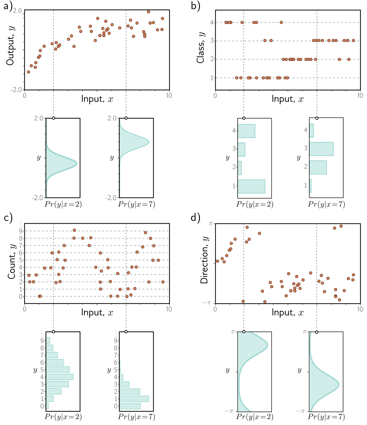
This also explains, in advance, why this chapter generalizes so easily. Nothing about a neural network needs to change to predict counts instead of temperatures. What changes is the distribution, and hence the loss.
3.1 Computing a distribution over outputs
Prince §5.1.1, p. 58.
A network outputs numbers, not distributions, so we need one more step. Choose a parametric distribution \(Pr(y \mid \boldsymbol{\theta})\) defined on the output domain, then use the network to compute one or more of its parameters \(\boldsymbol{\theta}\).
For a real-valued output \(y \in \mathbb{R}\) the univariate normal is a natural choice; it has parameters \(\boldsymbol{\theta} = \{\mu, \sigma^2\}\), and we might let the network predict the mean, \(\mu = \mathrm{f}[x, \boldsymbol{\phi}]\), and treat the variance \(\sigma^2\) as an unknown constant. The network’s job has been redefined, not made harder: the same piecewise linear function of \(x\) that used to be the prediction now indexes a family of distributions.
3.2 The maximum likelihood criterion
Prince §5.1.2, p. 58.
The model computes different distribution parameters \(\boldsymbol{\theta}_i = \mathbf{f}[\mathbf{x}_i, \boldsymbol{\phi}]\) for each training input. Each observed output \(y_i\) should be probable under its own distribution, so we choose the parameters that maximize the combined probability of all \(I\) training examples:
\[ \hat{\boldsymbol{\phi}} = \operatorname*{argmax}_{\boldsymbol{\phi}} \left[ \prod_{i=1}^{I} Pr(y_i \mid \mathbf{x}_i) \right] = \operatorname*{argmax}_{\boldsymbol{\phi}} \left[ \prod_{i=1}^{I} Pr\big(y_i \mid \mathbf{f}[\mathbf{x}_i, \boldsymbol{\phi}]\big) \right]. \tag{1}\]
Read as a function of \(y\), the quantity \(Pr(y \mid \boldsymbol{\psi})\) is a probability distribution and sums to one. Read as a function of the parameters \(\boldsymbol{\psi}\), it is a likelihood, and it does not generally sum to anything. Eq. 1 is the maximum likelihood criterion.
Two assumptions are hiding in that product, and both matter later.
- The data are identically distributed: the form of the distribution over outputs is the same for every data point. We use a normal at every \(x\), or a Bernoulli at every \(x\) — only the parameters change.
- The conditional distributions are independent given the inputs, so the total likelihood factorizes:
\[ Pr(y_1, y_2, \ldots, y_I \mid \mathbf{x}_1, \mathbf{x}_2, \ldots, \mathbf{x}_I) = \prod_{i=1}^{I} Pr(y_i \mid \mathbf{x}_i). \tag{2}\]
Together: the data are independent and identically distributed (i.i.d.). This is an assumption about the data collection, not about the network, and it is the first thing to question when a model behaves strangely on real engineering data — consecutive readings from one sensor, or parts from one production batch, are rarely independent.
3.3 Maximizing log-likelihood
Prince §5.1.3, p. 59; figure on p. 59.
Eq. 1 is unusable as written. Each factor is a probability, often much smaller than one, and the product of thousands of them cannot be represented in finite precision. Fortunately we can maximize the logarithm instead:
\[ \hat{\boldsymbol{\phi}} = \operatorname*{argmax}_{\boldsymbol{\phi}} \left[ \log\left[\prod_{i=1}^{I} Pr\big(y_i \mid \mathbf{f}[\mathbf{x}_i, \boldsymbol{\phi}]\big)\right] \right] = \operatorname*{argmax}_{\boldsymbol{\phi}} \left[ \sum_{i=1}^{I} \log\Big[ Pr\big(y_i \mid \mathbf{f}[\mathbf{x}_i, \boldsymbol{\phi}]\big) \Big] \right]. \tag{3}\]
This is equivalent, not merely similar, because the logarithm is monotonically increasing: if \(z > z'\) then \(\log[z] > \log[z']\) (fig. 2). Any change to \(\boldsymbol{\phi}\) that improves the likelihood improves the log-likelihood, and the two criteria have their maxima in exactly the same place. The practical gain is that a sum of logarithms is representable where a product of probabilities is not.
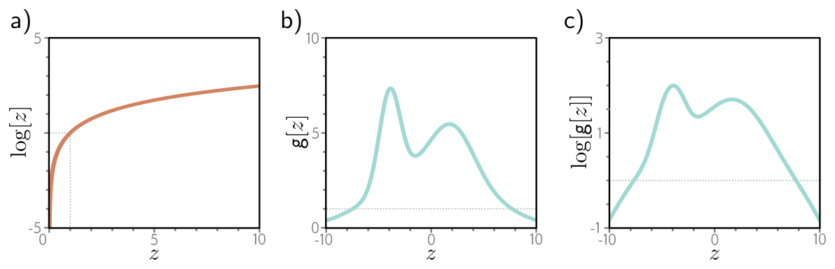
The failure this avoids is not subtle, and it is worth seeing once. Below, the “probabilities” are densities of standard normal residuals — none of them especially small on its own.
By five hundred examples the product has fallen into the subnormal range, and by two thousand it is exactly zero in double precision — and a gradient of zero tells the optimizer nothing. The sum of logarithms is perfectly well behaved at every size. Every deep learning framework works in log space for this reason, and you will meet the same trick again as logsumexp below.
3.4 Minimizing negative log-likelihood
Prince §5.1.4, p. 60.
By convention, model fitting is framed as minimization. Multiplying by minus one converts the maximum log-likelihood criterion into the negative log-likelihood criterion, and that is the loss:
\[ \hat{\boldsymbol{\phi}} = \operatorname*{argmin}_{\boldsymbol{\phi}} \left[ -\sum_{i=1}^{I} \log\Big[ Pr\big(y_i \mid \mathbf{f}[\mathbf{x}_i, \boldsymbol{\phi}]\big) \Big] \right] = \operatorname*{argmin}_{\boldsymbol{\phi}} \big[ L[\boldsymbol{\phi}] \big]. \tag{4}\]
3.5 Inference
Prince §5.1.5, p. 60.
The trained network no longer hands us an output; it hands us a distribution over outputs. Often we want a single number, so we return the maximum of that distribution:
\[ \hat{y} = \operatorname*{argmax}_{y} \Big[ Pr\big(y \mid \mathbf{f}[\mathbf{x}, \hat{\boldsymbol{\phi}}]\big) \Big]. \tag{5}\]
It is usually easy to express this in terms of the predicted parameters. For the univariate normal the maximum is at the mean \(\mu\), which is exactly what the network computed — so for regression this step is free. It will not always be.
4 The Recipe
Prince §5.2, p. 60.
Everything above collapses into four steps, and the rest of the chapter is nothing but this recipe applied three times.
The recipe for constructing a loss function
Given training data \(\{\mathbf{x}_i, y_i\}\):
- Choose a distribution. Pick a probability distribution \(Pr(y \mid \boldsymbol{\theta})\) defined over the domain of the predictions \(y\), with parameters \(\boldsymbol{\theta}\).
- Point the network at its parameters. Set the model \(\mathbf{f}[\mathbf{x}, \boldsymbol{\phi}]\) to predict one or more of them, so \(\boldsymbol{\theta} = \mathbf{f}[\mathbf{x}, \boldsymbol{\phi}]\) and \(Pr(y \mid \boldsymbol{\theta}) = Pr(y \mid \mathbf{f}[\mathbf{x}, \boldsymbol{\phi}])\).
- Train by minimizing the negative log-likelihood over the training pairs: \[ \hat{\boldsymbol{\phi}} = \operatorname*{argmin}_{\boldsymbol{\phi}} \left[ -\sum_{i=1}^{I} \log\Big[ Pr\big(y_i \mid \mathbf{f}[\mathbf{x}_i, \boldsymbol{\phi}]\big) \Big] \right]. \tag{6}\]
- Infer for a new test example \(\mathbf{x}\) by returning either the full distribution \(Pr(y \mid \mathbf{f}[\mathbf{x}, \hat{\boldsymbol{\phi}}])\) or its maximum.
Step 1 is the only place where judgement enters. Steps 2–4 are mechanical.
Note what step 2 does not say. The network is not required to predict all the distribution’s parameters. Which ones it predicts, and which are held fixed or learned as single global constants, is a modeling decision — and in §5.3 below, exactly that decision separates least squares from heteroscedastic regression.
5 Example 1: Univariate Regression
Prince §5.3, pp. 61–62; figures on pp. 61 and 63.
Predict a single real number \(y \in \mathbb{R}\) from input \(x\). Step 1: choose a distribution on \(\mathbb{R}\), and the univariate normal (fig. 3) is the obvious candidate. It has a mean \(\mu\), which locates the peak, and a variance \(\sigma^2\), whose positive root — the standard deviation — sets the width:
\[ Pr(y \mid \mu, \sigma^2) = \frac{1}{\sqrt{2\pi\sigma^2}} \exp\left[ \frac{-(y - \mu)^2}{2\sigma^2} \right]. \tag{7}\]
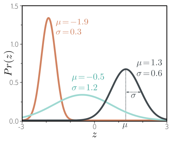
Step 2: let the network compute the mean, \(\mu = \mathrm{f}[x, \boldsymbol{\phi}]\), and leave the variance as a constant:
\[ Pr(y \mid \mathrm{f}[x, \boldsymbol{\phi}], \sigma^2) = \frac{1}{\sqrt{2\pi\sigma^2}} \exp\left[ \frac{-(y - \mathrm{f}[x, \boldsymbol{\phi}])^2}{2\sigma^2} \right]. \tag{8}\]
Step 3: the loss is the negative log-likelihood,
\[ L[\boldsymbol{\phi}] = -\sum_{i=1}^{I} \log\left[ \frac{1}{\sqrt{2\pi\sigma^2}} \exp\left[ \frac{-(y_i - \mathrm{f}[x_i, \boldsymbol{\phi}])^2}{2\sigma^2} \right] \right]. \tag{9}\]
5.1 The least squares loss function
Prince §5.3.1, p. 62.
Eq. 9 looks nothing like the criterion from Chapter 2, until you simplify it. Take the log inside:
\[ \begin{aligned} \hat{\boldsymbol{\phi}} &= \operatorname*{argmin}_{\boldsymbol{\phi}} \left[ -\sum_{i=1}^{I} \left( \log\left[\frac{1}{\sqrt{2\pi\sigma^2}}\right] - \frac{(y_i - \mathrm{f}[x_i, \boldsymbol{\phi}])^2}{2\sigma^2} \right) \right] \\ &= \operatorname*{argmin}_{\boldsymbol{\phi}} \left[ \sum_{i=1}^{I} \frac{(y_i - \mathrm{f}[x_i, \boldsymbol{\phi}])^2}{2\sigma^2} \right] = \operatorname*{argmin}_{\boldsymbol{\phi}} \left[ \sum_{i=1}^{I} \big(y_i - \mathrm{f}[x_i, \boldsymbol{\phi}]\big)^2 \right], \end{aligned} \tag{10}\]
where the first term was dropped because it does not depend on \(\boldsymbol{\phi}\), and the \(2\sigma^2\) because a positive constant scaling does not move the position of a minimum. What is left is the least squares loss of Chapter 2:
\[ L[\boldsymbol{\phi}] = \sum_{i=1}^{I} \big(y_i - \mathrm{f}[x_i, \boldsymbol{\phi}]\big)^2. \tag{11}\]
Fig. 4 makes the equivalence visual: panels (a) and (b) measure squared deviations for a good and a bad fit, and panels (c) and (d) measure the probability of the data under a normal distribution centred on the model’s prediction. They rank the two fits the same way because they are the same criterion.
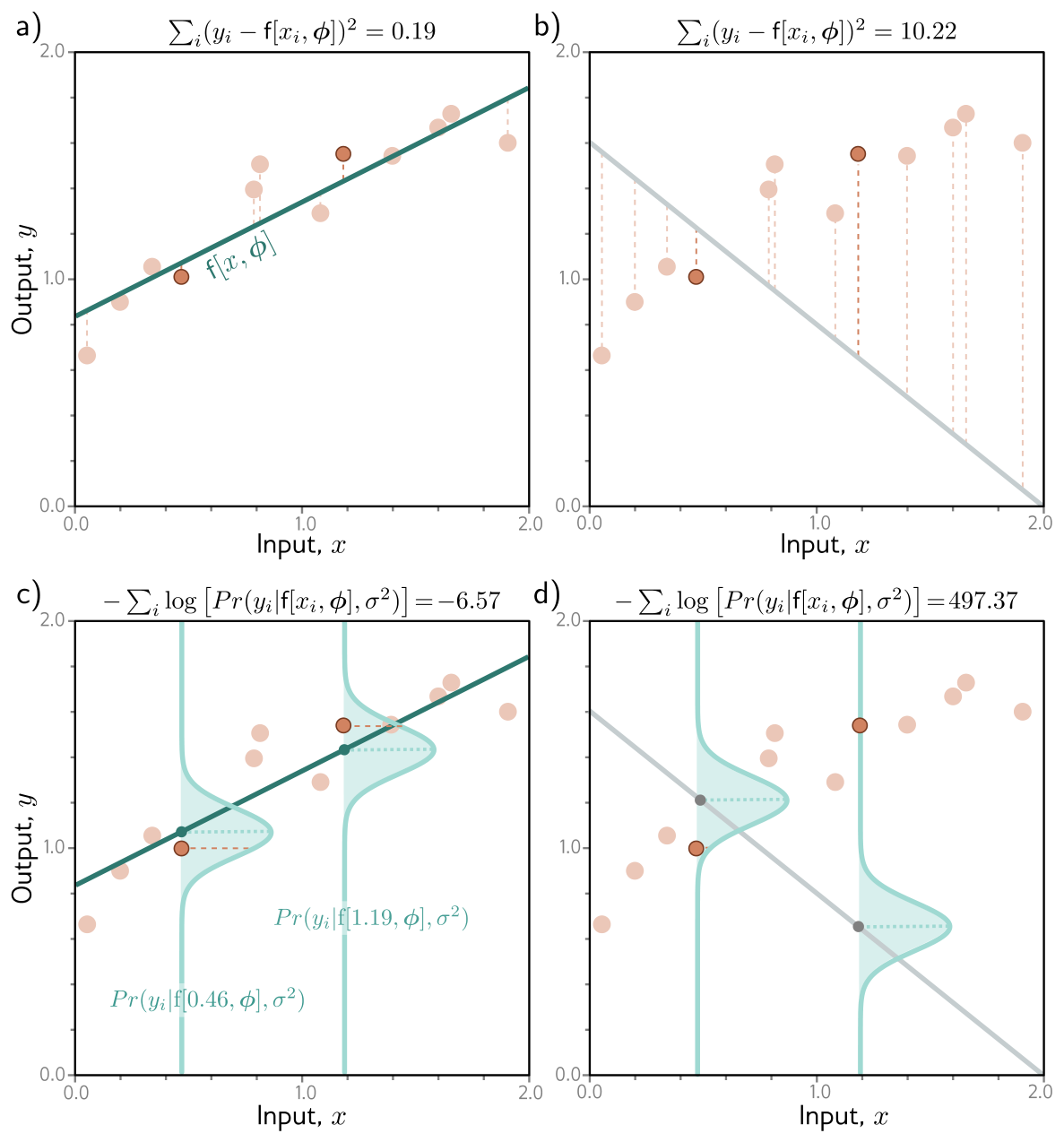
What least squares assumes
Least squares is not a neutral default. Eq. 10 shows it is exactly the negative log-likelihood under three assumptions: the errors are independent, they are normally distributed, and their variance is the same everywhere. When the errors have heavy tails, a squared penalty gives a single outlier enormous leverage — which is why a Laplace or \(t\) distribution, yielding an absolute-error loss, is the standard robust alternative. When the variance is not constant, §5.3.4 applies. Using least squares is a claim about your noise, whether or not you meant to make it.
We can check the algebra numerically. Because eq. 9 and eq. 11 differ only by the positive factor \(1/(2\sigma^2)\) and the additive constant \(\tfrac{I}{2}\log[2\pi\sigma^2]\), the two should agree to machine precision under that affine map, and their minima should coincide for any value of \(\sigma^2\).
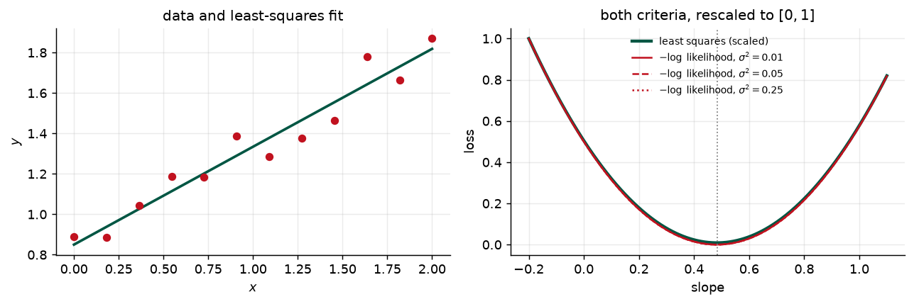
argmin slope, least squares: 0.4842

  sigma^2  argmin slope    max |NLL - (SSE/2s^2 + I/2 log 2 pi s^2)|
     0.01        0.4842                                     1.14e-13
     0.05        0.4842                                     1.42e-14
     0.25        0.4842                                     3.55e-15
The minima agree to the resolution of the grid and the two expressions agree to about \(10^{-14}\). Least squares really is the normal-distribution log-likelihood with the constants thrown away.
5.2 Inference
Prince §5.3.2, p. 62.
The network predicts \(\mu = \mathrm{f}[x, \boldsymbol{\phi}]\), so at inference
\[ \hat{y} = \operatorname*{argmax}_{y} \Big[ Pr\big(y \mid \mathrm{f}[x, \hat{\boldsymbol{\phi}}], \sigma^2\big) \Big] = \mathrm{f}[x, \hat{\boldsymbol{\phi}}]. \tag{12}\]
The maximum of a normal is at its mean, and the mean is what the network computed. Nothing to do.
5.3 Estimating the variance
Prince §5.3.3, pp. 62–64.
Eq. 11 does not mention \(\sigma^2\), which is convenient but throws information away. Nothing stops us treating \(\sigma^2\) as one more parameter and minimizing eq. 9 over both:
\[ \hat{\boldsymbol{\phi}}, \hat{\sigma}^2 = \operatorname*{argmin}_{\boldsymbol{\phi}, \sigma^2} \left[ -\sum_{i=1}^{I} \log\left[ \frac{1}{\sqrt{2\pi\sigma^2}} \exp\left[ \frac{-(y_i - \mathrm{f}[x_i, \boldsymbol{\phi}])^2}{2\sigma^2} \right] \right] \right]. \tag{13}\]
Now the model returns two things from one training run: the mean \(\mu = \mathrm{f}[x, \hat{\boldsymbol{\phi}}]\), which is the prediction, and \(\hat{\sigma}^2\), which quantifies how much to trust it. For an engineering model that second number is often the one the decision depends on.
5.4 Heteroscedastic regression
Prince §5.3.4, p. 64; figure on p. 65.
A single global \(\hat{\sigma}^2\) still assumes the noise is the same everywhere — homoscedastic. That is frequently wrong: a sensor is precise at low load and noisy at high load; a process is repeatable near its setpoint and erratic at the edge of its window. When the uncertainty varies with the input we call the model heteroscedastic.
The fix follows the recipe with no new ideas. Give the network two outputs, using \(\mathrm{f}_1[x, \boldsymbol{\phi}]\) for the mean and \(\mathrm{f}_2[x, \boldsymbol{\phi}]\) for the variance. One complication: a variance must be positive and a network output need not be, so we pass the second output through a function that maps \(\mathbb{R}\) to \(\mathbb{R}^+\). Squaring will do:
\[ \mu = \mathrm{f}_1[x, \boldsymbol{\phi}], \qquad \sigma^2 = \mathrm{f}_2[x, \boldsymbol{\phi}]^2, \tag{14}\]
giving the loss
\[ \hat{\boldsymbol{\phi}} = \operatorname*{argmin}_{\boldsymbol{\phi}} \left[ -\sum_{i=1}^{I} \left( \log\left[ \frac{1}{\sqrt{2\pi \mathrm{f}_2[x_i, \boldsymbol{\phi}]^2}} \right] - \frac{(y_i - \mathrm{f}_1[x_i, \boldsymbol{\phi}])^2}{2\,\mathrm{f}_2[x_i, \boldsymbol{\phi}]^2} \right) \right]. \tag{15}\]
Fig. 6 compares the two architectures and what they produce. In the homoscedastic model the mean is piecewise linear and the \(\pm 2\sigma\) band has constant width; in the heteroscedastic model the standard deviation is itself a piecewise linear function of \(x\) and the band breathes.
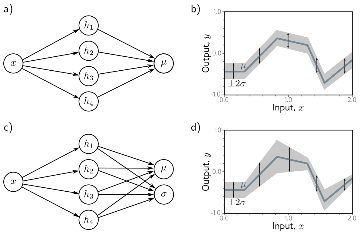
Notice that eq. 15 can no longer be simplified into least squares. The \(\log\) term survives because \(\mathrm{f}_2\) depends on \(\boldsymbol{\phi}\), and it is what stops the network from declaring infinite uncertainty everywhere: the squared-error term is divided by the variance, so widening the band cheapens the errors, while the \(\log\) term charges for the width. The loss balances the two, and that balance is exactly the maximum likelihood estimate.
Below we generate data whose noise grows with \(x\), fit both models with the same architecture and optimizer, and ask a question that squared error cannot answer: does the predicted uncertainty hold up?
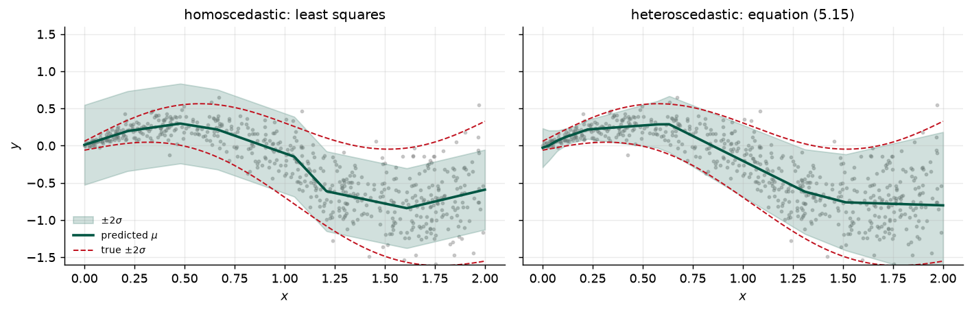
model                 mean NLL  in +/-2s, all   x < 0.7   x > 1.3
homoscedastic            0.104          93.8%    100.0%     85.3%
heteroscedastic         -0.140          96.5%     96.4%     95.7%
nominal for +/-2s                       95.5%     95.5%     95.5%

homoscedastic sigma: 0.269 everywhere
heteroscedastic sigma: 0.051 at the left edge, rising to 0.493 at the right
Both models find much the same mean — that part is least squares either way. The difference is in the interval. Averaged over all the data the homoscedastic band looks almost respectable, which is the trap: it is far too conservative where the process is quiet and it under-covers exactly where the process is noisy and a wrong answer costs the most. The heteroscedastic model is close to nominal in both halves. If your model’s output feeds a tolerance decision, this is the difference between a useful interval and a decorative one.
6 Example 2: Binary Classification
Prince §5.4, pp. 64–66; figures on pp. 65–67.
Now assign the input to one of two classes, \(y \in \{0, 1\}\), where \(y\) is called a label. Predicting whether a review is positive, whether a tumor is present, whether a weld will pass inspection — same recipe, different distribution.
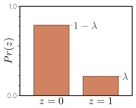
Step 1: the Bernoulli distribution is defined on \(\{0, 1\}\) and has one parameter \(\lambda \in [0, 1]\), the probability that \(y = 1\) (fig. 8):
\[ Pr(y \mid \lambda) = \begin{cases} 1 - \lambda & y = 0 \\ \lambda & y = 1, \end{cases} \tag{16}\]
which can be written in one line as
\[ Pr(y \mid \lambda) = (1 - \lambda)^{1 - y} \cdot \lambda^{y}. \tag{17}\]
Step 2: have the network predict \(\lambda\). But \(\lambda\) must lie in \([0, 1]\) and a network output is an arbitrary real number, so we pass it through a squashing function. The logistic sigmoid (fig. 9) does the job:
\[ \mathrm{sig}[z] = \frac{1}{1 + \exp[-z]}. \tag{18}\]
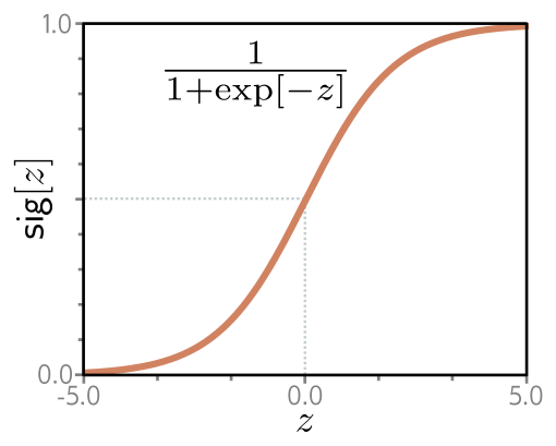
So \(\lambda = \mathrm{sig}[\mathrm{f}[x, \boldsymbol{\phi}]]\) and the likelihood is
\[ Pr(y \mid x) = \big(1 - \mathrm{sig}[\mathrm{f}[x, \boldsymbol{\phi}]]\big)^{1-y} \cdot \mathrm{sig}[\mathrm{f}[x, \boldsymbol{\phi}]]^{y}. \tag{19}\]
Step 3: the loss is the negative log-likelihood of the training set,
\[ L[\boldsymbol{\phi}] = \sum_{i=1}^{I} -(1 - y_i) \log\Big[ 1 - \mathrm{sig}[\mathrm{f}[x_i, \boldsymbol{\phi}]] \Big] - y_i \log\Big[ \mathrm{sig}[\mathrm{f}[x_i, \boldsymbol{\phi}]] \Big], \tag{20}\]
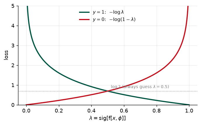
known — for reasons that §5.7 will supply — as the binary cross-entropy loss. The indicator structure is worth reading carefully: for a positive example only the second term survives and the loss is \(-\log \lambda\); for a negative example only the first survives and it is \(-\log(1 - \lambda)\).
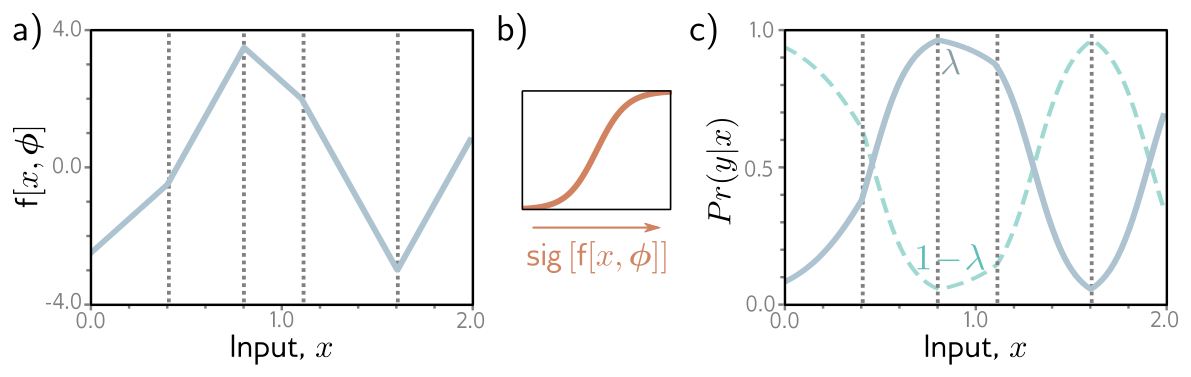
Step 4: the transformed output is the probability that \(y = 1\). For a point estimate we set \(y = 1\) if \(\lambda > 0.5\) and \(y = 0\) otherwise — though note that the threshold is a separate decision from the model, and \(0.5\) is only right when the two kinds of error cost the same.
Fig. 11 is our version of fig. 10. The helper in the first cell turns any piecewise linear function specified by its knots into a shallow ReLU network, which is a constructive restatement of Week 3: on a bounded interval, every continuous piecewise linear function is a shallow network.
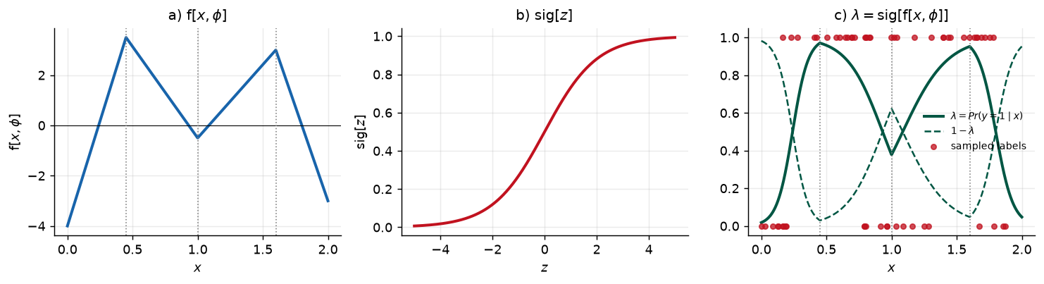
36 of 60 sampled labels are positive

model                         total loss  per example
the true lambda[x]                27.238        0.454
a constant lambda = 0.5           41.589        0.693

accuracy of thresholding lambda at 0.5: 75.0%
The comparison in the last two lines is the one to remember. A model that predicts \(\lambda = 0.5\) for everything — the coin flip — pays \(\log 2 \approx 0.693\) nats per example. Any loss below that means the model has learned something; a loss above it means the model is worse than knowing nothing, which is possible, because confident wrong answers are punished without limit.
That unboundedness is visible in the per-example loss, which is problem 5.2.
7 Example 3: Multiclass Classification
Prince §5.5, pp. 67–69; figures on pp. 67–68.
With \(K > 2\) classes, \(y \in \{1, 2, \ldots, K\}\): which of ten digits is in this image, which of many words comes next, which of six failure modes this vibration signature indicates.
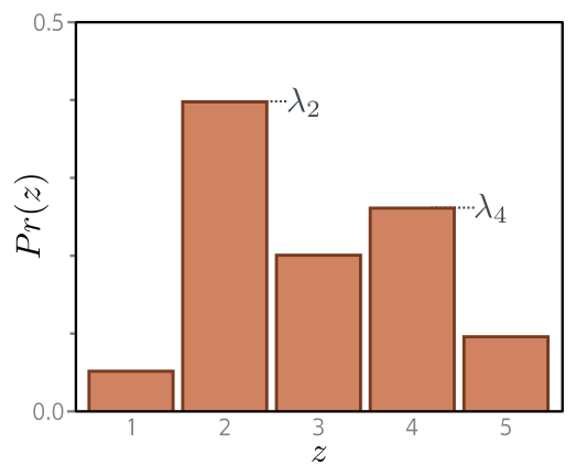
Step 1: the categorical distribution (fig. 13) is defined on exactly this domain. It has \(K\) parameters,
\[ Pr(y = k) = \lambda_k, \tag{21}\]
each constrained to \([0, 1]\), and together they must sum to one.
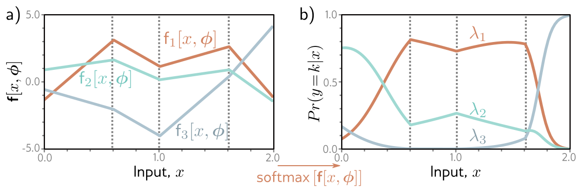
Step 2: use a network with \(K\) outputs. Again the raw outputs — the logits — will not respect the constraints, so we pass them through the softmax function, which takes an arbitrary vector of length \(K\) and returns one of the same length whose entries are in \([0, 1]\) and sum to one:
\[ \mathrm{softmax}_k[\mathbf{z}] = \frac{\exp[z_k]}{\sum_{k'=1}^{K} \exp[z_{k'}]}. \tag{22}\]
The exponentials guarantee positivity; the denominator guarantees the sum. The likelihood is then
\[ Pr(y = k \mid \mathbf{x}) = \mathrm{softmax}_k\big[ \mathbf{f}[\mathbf{x}, \boldsymbol{\phi}] \big], \tag{23}\]
and step 3 gives the multiclass cross-entropy loss:
\[ L[\boldsymbol{\phi}] = -\sum_{i=1}^{I} \log\Big[ \mathrm{softmax}_{y_i}\big[ \mathbf{f}[\mathbf{x}_i, \boldsymbol{\phi}] \big] \Big] = -\sum_{i=1}^{I} \left( \mathrm{f}_{y_i}[\mathbf{x}_i, \boldsymbol{\phi}] - \log\left[ \sum_{k'=1}^{K} \exp\big[\mathrm{f}_{k'}[\mathbf{x}_i, \boldsymbol{\phi}]\big] \right] \right). \tag{24}\]
The second form is the one that gets implemented. It never forms the softmax explicitly: it takes the logit of the correct class and subtracts a logsumexp over all the logits. Step 4, inference, takes the most probable category, \(\hat{y} = \operatorname{argmax}_k[Pr(y = k \mid \mathbf{f}[\mathbf{x},
\hat{\boldsymbol{\phi}}])]\) — whichever curve is highest at that \(x\) in fig. 14.
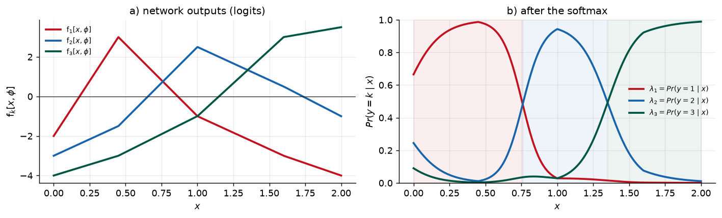
every column of the softmax sums to one: True
classes that are ever the argmax       : [1, 2, 3]
Two properties of the softmax are worth knowing before you use it.
softmax is invariant to adding a constant to every logit:
   z +     0.0: [0.291763 0.058906 0.649331]
   z +     5.0: [0.291763 0.058906 0.649331]
   z +  -100.0: [0.291763 0.058906 0.649331]

=> the K logits carry only K - 1 degrees of freedom; the model can never
   identify their absolute level, only their differences.

the exponentials overflow if you implement equation (5.22) literally:
   exp[z] / sum exp[z] with z = [1000. 1001.  999.]  ->  [nan nan nan]
   subtracting max[z] first                       ->  [0.244728 0.665241 0.090031]
   log Pr(y = 2) by log-sum-exp, equation (5.24)  ->  -0.407606   (= log 0.665241)
Shift invariance is why a softmax layer with \(K\) outputs is over-parameterized, and the overflow is why eq. 24 is implemented in its second, logsumexp form. torch.nn.CrossEntropyLoss does both for you, which is the main reason you should not build your own.
7.1 Predicting other data types
Prince §5.5.1, p. 69; figure on p. 70.
Regression and classification cover most of what we will do, but the recipe does not care. To predict something else, pick a distribution defined on that domain and turn the crank. Prince’s figure 5.11 tabulates the standard choices; it is reproduced here as a table.
| Data type | Domain | Distribution | Use |
|---|---|---|---|
| univariate, continuous, unbounded | \(y \in \mathbb{R}\) | univariate normal | regression |
| univariate, continuous, unbounded | \(y \in \mathbb{R}\) | Laplace or \(t\) | robust regression |
| univariate, continuous, unbounded | \(y \in \mathbb{R}\) | mixture of Gaussians | multimodal regression |
| univariate, continuous, bounded below | \(y \in \mathbb{R}^+\) | exponential or gamma | predicting magnitude |
| univariate, continuous, bounded | \(y \in [0, 1]\) | beta | predicting proportions |
| multivariate, continuous, unbounded | \(y \in \mathbb{R}^K\) | multivariate normal | multivariate regression |
| univariate, continuous, circular | \(y \in (-\pi, \pi]\) | von Mises | predicting direction |
| univariate, discrete, binary | \(y \in \{0, 1\}\) | Bernoulli | binary classification |
| univariate, discrete, bounded | \(y \in \{1, 2, \ldots, K\}\) | categorical | multiclass classification |
| univariate, discrete, bounded below | \(y \in \{0, 1, 2, \ldots\}\) | Poisson | predicting event counts |
| multivariate, discrete, permutation | \(y \in \mathrm{Perm}[1, 2, \ldots, K]\) | Plackett-Luce | ranking |
Every row is a homework problem waiting to happen, and problems 5.3–5.6 at the end of the chapter walk through four of them. The pattern never changes: write down the density, take \(-\log\), sum over the data, and decide which parameters the network computes and which are constants.
8 Multiple Outputs
Prince §5.6, pp. 69–70.
Often we want more than one prediction from the same model: a molecule’s melting and boiling point, or a class label at every pixel of an image. It is possible to define a multivariate distribution and have the network predict its parameters, but the usual move is to assume the predictions are independent given the input, so the probability factorizes over the elements \(y_d\) of \(\mathbf{y}\):
\[ Pr(\mathbf{y} \mid \mathbf{f}[\mathbf{x}, \boldsymbol{\phi}]) = \prod_d Pr\big(y_d \mid \mathbf{f}_d[\mathbf{x}, \boldsymbol{\phi}]\big), \tag{25}\]
where \(\mathbf{f}_d[\mathbf{x}, \boldsymbol{\phi}]\) is the \(d\)th set of network outputs — the parameters of the distribution over \(y_d\). Take the negative logarithm and the product becomes a sum:
\[ L[\boldsymbol{\phi}] = -\sum_{i=1}^{I} \sum_d \log\Big[ Pr\big(y_{id} \mid \mathbf{f}_d[\mathbf{x}_i, \boldsymbol{\phi}]\big) \Big]. \tag{26}\]
The same argument covers predictions of different kinds from one network. To predict wind direction and wind speed, use a von Mises distribution for the direction and an exponential for the speed; independence makes the joint likelihood a product, and the negative log-likelihood a sum of two terms.
The hidden weighting problem
Eq. 26 adds the terms with weight one each, which looks neutral and is not. The relative size of the terms depends on the units and the scale of each output, so a network predicting a person’s height in meters and weight in kilograms will effectively ignore the height (problem 5.9). Maximum likelihood gives a principled answer — if each dimension gets its own estimated variance, as in eq. 14, the terms are automatically weighted by how predictable each output is. Otherwise you are choosing weights by accident. Standardizing every output to zero mean and unit variance before training is the cheap fix.
9 Cross-Entropy Loss
Prince §5.7, pp. 71–72; figure on p. 71.
Everything so far has been built from negative log-likelihood, yet the losses in §5.4 and §5.5 are universally called cross-entropy. The two names describe the same object, and this section shows why.
The cross-entropy view starts somewhere else: find the model distribution \(Pr(y \mid \boldsymbol{\theta})\) that is closest to the empirical distribution \(q(y)\) of the observed data (fig. 16). Distance between distributions is measured by the Kullback-Leibler divergence,
\[ D_{KL}\big[q \,\|\, p\big] = \int_{-\infty}^{\infty} q(z) \log\big[q(z)\big] \, dz - \int_{-\infty}^{\infty} q(z) \log\big[p(z)\big] \, dz. \tag{27}\]
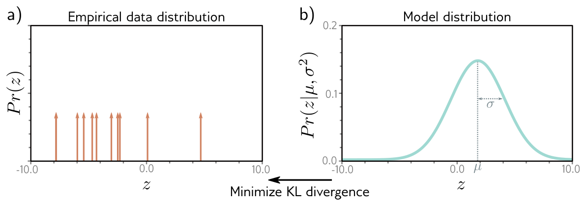
The empirical distribution of a finite sample \(\{y_i\}_{i=1}^{I}\) is a set of point masses,
\[ q(y) = \frac{1}{I} \sum_{i=1}^{I} \delta[y - y_i], \tag{28}\]
with \(\delta[\bullet]\) the Dirac delta. Minimizing the KL divergence between the model and this empirical distribution,
\[ \hat{\boldsymbol{\theta}} = \operatorname*{argmin}_{\boldsymbol{\theta}} \left[ -\int_{-\infty}^{\infty} q(y) \log\big[Pr(y \mid \boldsymbol{\theta})\big] \, dy \right], \tag{29}\]
drops the first term of eq. 27 because it has no dependence on \(\boldsymbol{\theta}\). What remains is the cross-entropy. Substituting eq. 28 and using the sifting property of the delta,
\[ \hat{\boldsymbol{\theta}} = \operatorname*{argmin}_{\boldsymbol{\theta}} \left[ -\frac{1}{I} \sum_{i=1}^{I} \log\big[Pr(y_i \mid \boldsymbol{\theta})\big] \right] = \operatorname*{argmin}_{\boldsymbol{\theta}} \left[ -\sum_{i=1}^{I} \log\big[Pr(y_i \mid \boldsymbol{\theta})\big] \right], \tag{30}\]
where the constant \(1/I\) goes because it does not move the minimum. Since the distribution parameters are computed by the model, \(\boldsymbol{\theta} = \mathbf{f}[\mathbf{x}_i, \boldsymbol{\phi}]\),
\[ \hat{\boldsymbol{\phi}} = \operatorname*{argmin}_{\boldsymbol{\phi}} \left[ -\sum_{i=1}^{I} \log\Big[ Pr\big(y_i \mid \mathbf{f}[\mathbf{x}_i, \boldsymbol{\phi}]\big) \Big] \right], \tag{31}\]
which is eq. 4 exactly. Maximizing the likelihood of the data and minimizing the distance from the empirical distribution are the same procedure, reached from opposite directions.
The discrete case makes the bookkeeping visible in a few lines.
empirical q               : [0.552 0.22  0.136 0.092]
model p                   : [0.4 0.3 0.2 0.1]

cross-entropy H[q, p]     : 1.201388
negative log-likelihood/I : 1.201388   <- the same number

entropy H[q]              : 1.151953
KL[q || p] = H[q,p] - H[q]: 0.049435   >= 0, zero only when p = q

H[q, q], i.e. the best any model could do on this sample: 1.151953
The cross-entropy decomposes as \(H[q, p] = H[q] + D_{KL}[q \,\|\, p]\). The first term is a property of the data alone and no model can reduce it; the second is what training minimizes. A cross-entropy of \(1.20\) nats therefore does not mean the model is bad — \(1.15\) of it is irreducible, and training can only ever recover the remaining \(0.05\). This is also the cleanest reason the loss value on its own is a poor progress report, and why Chapter 8 will insist on comparing against a baseline.
10 Losses in PyTorch
Ours; UDL notebooks 5.1–5.3.
Three lines of PyTorch cover this entire chapter, and each corresponds to one equation above.
| Prediction type | Equation | PyTorch | Expects |
|---|---|---|---|
| univariate regression | eq. 11 | nn.MSELoss |
prediction and target |
| binary classification | eq. 20 | nn.BCEWithLogitsLoss |
logits and \(\{0,1\}\) target |
| multiclass classification | eq. 24 | nn.CrossEntropyLoss |
logits and integer class index |
The first check is that they really are the equations, with no hidden constants beyond the choice of reduction.
loss                         PyTorch   our equation   equation
MSELoss                    14.962182      14.962182     (5.11)
BCEWithLogitsLoss           6.674289       6.674290     (5.20)
CrossEntropyLoss           15.339268      15.339268     (5.24)
The second check is the one that costs people a day of debugging. BCELoss takes probabilities and BCEWithLogitsLoss takes logits; they compute the same quantity in exact arithmetic, and they do not behave the same in floating point.
  logit z   BCELoss(sigmoid(z))   BCEWithLogitsLoss(z)   exact -log sig[z]   dL/dz, BCELoss  dL/dz, logits
       -5                5.0067                 5.0067              5.0000          -0.9933        -0.9933
      -20               20.0000                20.0000             20.0000          -1.0000        -1.0000
      -80               80.0000                80.0000             80.0000          -0.0000        -1.0000
     -200              100.0000               200.0000            200.0000          -0.0000        -1.0000
     -500              100.0000               500.0000            500.0000          -0.0000        -1.0000
Read the gradient columns. By \(z = -80\) the sigmoid has underflowed to zero in float32, so BCELoss sees \(\log[0]\), returns a clamped value, and reports a gradient of zero — the worst possible failure, because the loss still looks plausible while the example has silently stopped contributing to training. The logit version keeps the exact answer, \(L = -z\) with \(dL/dz = -1\), at every magnitude. The same argument applies to CrossEntropyLoss, which is why it takes logits and not the output of a Softmax layer.
Three rules that follow from this chapter
- Never put a sigmoid or softmax at the end of a network that feeds
BCEWithLogitsLossorCrossEntropyLoss. They apply it internally, in log space. Applying it twice is both wrong and numerically fragile. reductionchanges the effective learning rate, not the model.sumis eq. 11 literally;meandivides by \(I\) and is the default because it makes the gradient magnitude independent of batch size.- Add the sigmoid or softmax back at inference time, when you want a probability rather than a loss.
11 Summary
Prince §5.8, pp. 72–73.
We stopped thinking of a network as predicting outputs \(y\) from data \(\mathbf{x}\) and started thinking of it as computing the parameters \(\boldsymbol{\theta}\) of a probability distribution \(Pr(y \mid \boldsymbol{\theta})\) over the output space. Choosing the parameters \(\boldsymbol{\phi}\) that maximize the likelihood of the observed data — equivalently, that minimize the negative log-likelihood — turns the choice of a loss function from a matter of taste into a consequence of one modeling decision: which distribution fits the output domain.
Least squares follows from assuming \(y\) is normally distributed with constant variance and that the network predicts the mean. Letting the network predict the variance as well gives an uncertainty estimate; letting that variance depend on the input gives the heteroscedastic model. The same recipe with a Bernoulli distribution and a logistic sigmoid gives binary cross-entropy, and with a categorical distribution and a softmax gives multiclass cross-entropy. Multiple outputs are handled by assuming independence, which turns a product of likelihoods into a sum of losses. Finally, the cross-entropy criterion — minimizing the KL divergence between the model and the empirical data distribution — turns out to be the negative log-likelihood criterion under another name.
Next: we now have a family of functions (Weeks 3 and 4) and a single number that says how well any member of it describes the data (this week). What we do not have is a way to find the member that minimizes that number. Chapter 6 introduces gradient descent and its stochastic variants, and Chapter 7 explains how to compute the gradients a network of many layers needs.
12 Exercises
1. (UDL 5.1 and 5.2) Show that the logistic sigmoid \(\mathrm{sig}[z] = 1 / (1 + \exp[-z])\) maps \(z = -\infty\) to \(0\), \(z = 0\) to \(0.5\), and \(z = \infty\) to \(1\). Then, for the single-example binary loss of eq. 20, plot the loss against the transformed output \(\mathrm{sig}[\mathrm{f}[x, \boldsymbol{\phi}]] \in [0, 1]\) for \(y = 0\) and for \(y = 1\), and confirm your sketch against fig. 12. What is the loss of a model that always answers \(\lambda = 0.5\), and why is that number a useful baseline?
2. Derive eq. 11 from eq. 9 in full, justifying each dropped term. Then state the three assumptions least squares encodes, and for each one give a measurement situation from your own field where it fails.
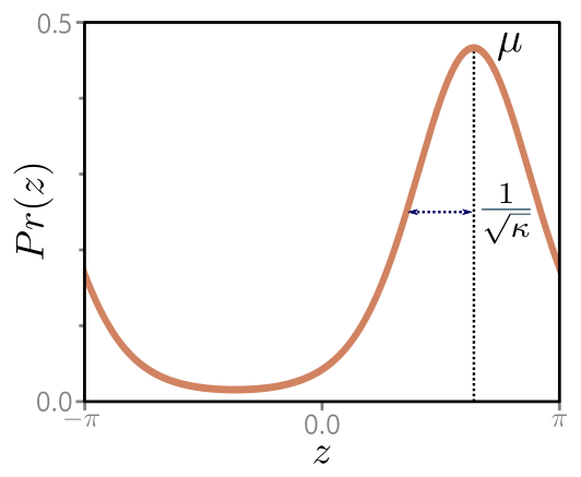
3. (UDL 5.3*) Predict the direction \(y\) in radians of the prevailing wind from barometric pressure \(x\). A suitable distribution on a circular domain is the von Mises (fig. 17), \[ Pr(y \mid \mu, \kappa) = \frac{\exp\big[\kappa \cos[y - \mu]\big]}{2\pi \cdot \mathrm{Bessel}_0[\kappa]}, \] where \(\mu\) is the mean direction and \(\kappa\) the concentration. Use the recipe of §5.2 to build a loss function for a model \(\mathrm{f}[x, \boldsymbol{\phi}]\) that predicts \(\mu\), treating \(\kappa\) as constant. How would you perform inference?
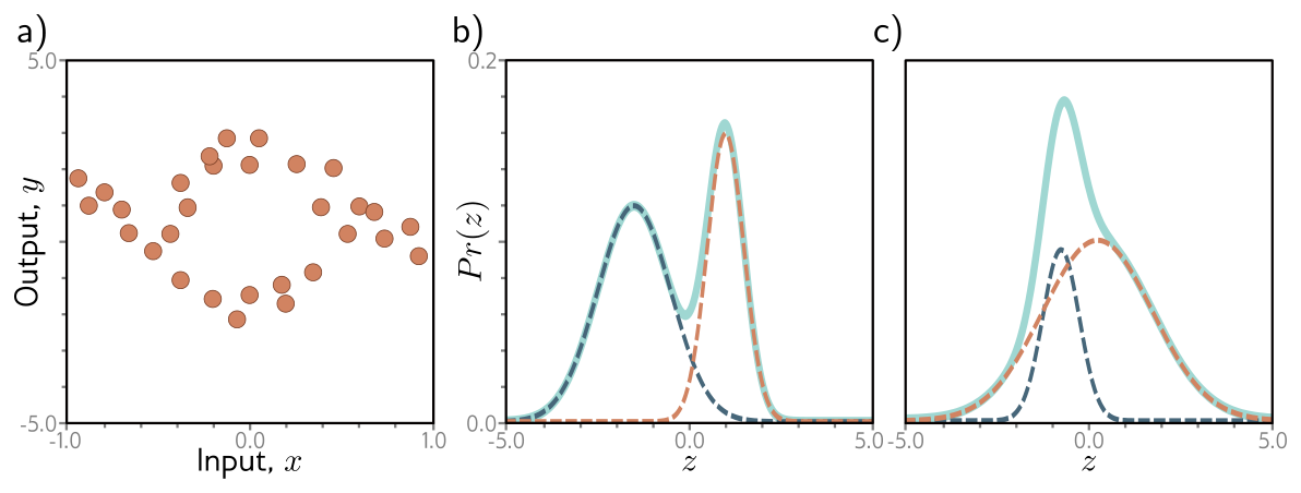
4. (UDL 5.4* and 5.5) Sometimes there is more than one valid output for a given input (fig. 18a). A mixture of two Gaussians with parameters \(\boldsymbol{\theta} = \{\lambda, \mu_1, \sigma_1^2, \mu_2, \sigma_2^2\}\), \[ Pr(y \mid \boldsymbol{\theta}) = \frac{\lambda}{\sqrt{2\pi\sigma_1^2}} \exp\left[\frac{-(y - \mu_1)^2}{2\sigma_1^2}\right] + \frac{1 - \lambda}{\sqrt{2\pi\sigma_2^2}} \exp\left[\frac{-(y - \mu_2)^2}{2\sigma_2^2}\right], \] can represent it. Construct a loss for a model that predicts this mixture from \(I\) training pairs. How many outputs does the network need, and what must you do to each one to keep the parameters valid? What problems do you foresee at inference time, and why does eq. 5 stop being easy here? Then extend problem 3 to a mixture of two von Mises distributions and write the likelihood.
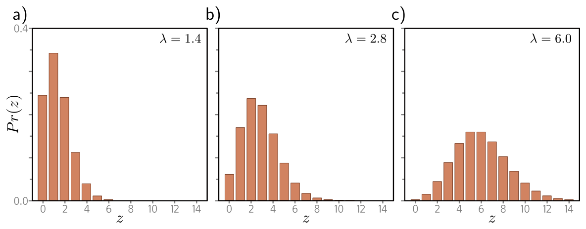
5. (UDL 5.6) Predict the number of pedestrians \(y \in \{0, 1, 2, \ldots\}\) passing a point in the next minute from data \(x\) describing time of day, position, and neighborhood type. A suitable distribution for counts is the Poisson (fig. 19), with rate \(\lambda > 0\) and \[ Pr(y = k) = \frac{\lambda^k e^{-\lambda}}{k!}. \] Design the loss function for \(I\) training pairs. Which term can be dropped during optimization, and why? What function would you use to keep the network’s output positive, and what would go wrong with the squaring used in eq. 14?
6. (UDL 5.7 and 5.9*) Consider a multivariate regression predicting ten outputs, \(\mathbf{y} \in \mathbb{R}^{10}\), each modeled with an independent normal whose mean is predicted by the network and whose variance \(\sigma^2\) is a shared constant. Write \(Pr(\mathbf{y} \mid \mathbf{f}[\mathbf{x}, \boldsymbol{\phi}])\) and show that minimizing the negative log-likelihood is still a sum of squared terms. Then suppose two of those outputs are a person’s height in meters and their weight in kilograms. What goes wrong, and what are two ways to fix it? Relate your answer to the callout in Section 8.
7. (UDL 5.8* and 5.10) Construct a loss for multivariate predictions \(\mathbf{y} \in \mathbb{R}^{D_o}\) using independent normals with a different variance \(\sigma_d^2\) per dimension, where both the means and the variances vary with the input. How many outputs does the network need? Then extend problem 3 to predict wind direction and wind speed together, naming the distribution you choose for each and writing the combined loss.
8. A bolted joint on an assembly line is inspected and recorded as pass or fail, and 3% of joints fail. A colleague trains a classifier with BCEWithLogitsLoss, reports 97.2% accuracy, and proposes deploying it. (a) Using fig. 12, explain what loss value a model that always predicts “pass” would achieve, and why accuracy is the wrong number to quote here. (b) The chapter notes (p. 73) describe focal loss for exactly this situation. Explain in terms of eq. 20 what “down-weighting well-classified examples” does to the gradient. (c) Propose a threshold other than \(0.5\) and justify it from the relative cost of the two errors, not from the model.
9. Computational. The heteroscedastic cell fits a two-output network with eq. 15. In the notebook: (a) replace the squaring in eq. 14 with \(\sigma^2 = \exp[\mathrm{f}_2[x, \boldsymbol{\phi}]]\) and compare the fitted \(\sigma\) curves and the coverage table; (b) remove the \(\log\) term from eq. 15, retrain, and report what the network does to \(\sigma\) and why; (c) drop the \(10^{-6}\) floor on the variance and describe the failure. Explain each result in terms of the two competing terms of eq. 15.
10. Computational. Take the three-class model of fig. 15 and treat its softmax outputs as the true label distribution. Sample 400 labels from it. Then (a) fit a small network with CrossEntropyLoss and compare its achieved loss with \(H[q]\) computed from the true conditional distributions — this is the irreducible floor; (b) add a constant of 50 to every logit of the trained network’s last layer and confirm that neither the loss nor the predictions change; (c) replace CrossEntropyLoss with NLLLoss applied to log(softmax(...)) computed naively, scale the logits up by a factor of 200, and report the first magnitude at which the two disagree.
13 Textbook Reference Map
Every part of this page, mapped to Prince, Understanding Deep Learning (MIT Press, 2024) (Prince 2024). Page numbers are those of the printed book.
| This page | Prince section | Pages | Figures used |
|---|---|---|---|
| What a Loss Function Is For | Ch. 5 opening | 56 | — |
| From Predictions to Distributions | §5.1 | 56–57 | 5.1 (p. 57) |
| — Computing a distribution over outputs | §5.1.1 | 58 | — |
| — The maximum likelihood criterion | §5.1.2 | 58 | — |
| — Maximizing log-likelihood | §5.1.3 | 59 | 5.2 (p. 59) |
| — Minimizing negative log-likelihood | §5.1.4 | 60 | — |
| — Inference | §5.1.5 | 60 | — |
| The Recipe | §5.2 | 60 | — |
| Example 1: Univariate Regression | §5.3 | 61–62 | 5.3 (p. 61) |
| — The least squares loss function | §5.3.1 | 62 | 5.4 (p. 63) |
| — Inference | §5.3.2 | 62 | — |
| — Estimating the variance | §5.3.3 | 62–64 | — |
| — Heteroscedastic regression | §5.3.4 | 64 | 5.5 (p. 65) |
| Example 2: Binary Classification | §5.4 | 64–66 | 5.6 (p. 65), 5.7 (p. 66), 5.8 (p. 67) |
| Example 3: Multiclass Classification | §5.5 | 67–69 | 5.9 (p. 67), 5.10 (p. 68) |
| — Predicting other data types | §5.5.1 | 69 | 5.11 (p. 70), as a table |
| Multiple Outputs | §5.6 | 69–70 | — |
| Cross-Entropy Loss | §5.7 | 71–72 | 5.12 (p. 71) |
| Losses in PyTorch | ours; notebooks 5.1–5.3 | — | — |
| Summary | §5.8 | 72–73 | — |
| Exercises 1, 3–7 | Problems 5.1–5.10 | 74–76 | 5.13 (p. 74), 5.14 (p. 75), 5.15 (p. 76) |
Equations on this page correspond to Prince as follows: eq. 1 is his (5.1), eq. 2 is (5.2), eq. 3 is (5.3), eq. 4 is (5.4), eq. 5 is (5.5), eq. 6 is (5.6), eq. 7 is (5.7), eq. 8 is (5.8), eq. 9 is (5.9), eq. 10 is (5.10), eq. 11 is (5.11), eq. 12 is (5.12), eq. 13 is (5.13), eq. 14 is (5.14), eq. 15 is (5.15), eq. 16 is (5.16), eq. 17 is (5.17), eq. 18 is (5.18), eq. 19 is (5.19), eq. 20 is (5.20), eq. 21 is (5.21), eq. 22 is (5.22), eq. 23 is (5.23), eq. 24 is (5.24), eq. 25 is (5.25), eq. 26 is (5.26), eq. 27 is (5.27), eq. 28 is (5.28), eq. 29 is (5.29), eq. 30 is (5.30), and eq. 31 is (5.31). The von Mises, mixture-of-Gaussians, and Poisson densities in the exercises are his (5.34), (5.35), and (5.36).
Figure credits
Figures 5.1–5.15 are reproduced unaltered from Prince, Understanding Deep Learning (MIT Press, 2024), which is distributed under a Creative Commons CC-BY-NC-ND license, and are used here for non-commercial classroom instruction. Figure 5.11 is reproduced as a table with its contents unchanged. All other figures on this page are generated by the code in this week’s notebook.
14 Further Reading
- Prince, Understanding Deep Learning, Chapter 5 (Prince 2024) — the assigned reading. The chapter notes (pp. 73–74) survey robust regression, quantile regression, class imbalance, learning to rank, and the non-probabilistic losses this chapter sets aside.
- ▶ UDL notebooks 5.1–5.3 — Prince’s own Colab notebooks for this chapter; links to each are at the top of this page.
- ▶ This week’s notebook — every cell above, in one Colab file.
- Nix & Weigend (1994) (Nix and Weigend 1994) — the original heteroscedastic neural network: two outputs, mean and variance, trained on eq. 15.
- Kendall & Gal (2017) (Kendall and Gal 2017) — the modern treatment of the same idea, and the distinction between noise in the data and uncertainty in the model.
- Bishop (1994) (Bishop 1994) — mixture density networks, the general form of problem 4.
- Koenker & Hallock (2001) (Koenker and Hallock 2001) — quantile regression, for when you need “the value will be below this 90% of the time” rather than a mean.
- Lin et al. (2017) (Lin et al. 2017) — focal loss, the standard remedy for the class imbalance of exercise 8.
- Guo et al. (2017) (Guo et al. 2017) — modern networks minimize cross-entropy well and are still badly calibrated; required reading before you treat a softmax output as a probability.
- Goodfellow, Bengio & Courville, Deep Learning, §5.5 and §6.2 (Goodfellow, Bengio, and Courville 2016) — maximum likelihood estimation and output units, a second pass over the same material.
References
Bishop, Christopher M. 1994. “Mixture Density Networks.” NCRG/94/004. Aston University.
Goodfellow, Ian, Yoshua Bengio, and Aaron Courville. 2016. Deep Learning. MIT Press. https://www.deeplearningbook.org/.
Guo, Chuan, Geoff Pleiss, Yu Sun, and Kilian Q. Weinberger. 2017. “On Calibration of Modern Neural Networks.” In International Conference on Machine Learning, 1321–30.
Kendall, Alex, and Yarin Gal. 2017. “What Uncertainties Do We Need in Bayesian Deep Learning for Computer Vision?” In Advances in Neural Information Processing Systems, 5574–84.
Koenker, Roger, and Kevin F. Hallock. 2001. “Quantile Regression.” Journal of Economic Perspectives 15 (4): 143–56.
Lin, Tsung-Yi, Priya Goyal, Ross Girshick, Kaiming He, and Piotr Dollár. 2017. “Focal Loss for Dense Object Detection.” In IEEE International Conference on Computer Vision, 2980–88.
Nix, David A., and Andreas S. Weigend. 1994. “Estimating the Mean and Variance of the Target Probability Distribution.” In IEEE International Conference on Neural Networks, 55–60.
Prince, Simon J. D. 2024. Understanding Deep Learning. MIT Press. https://udlbook.github.io/udlbook/.