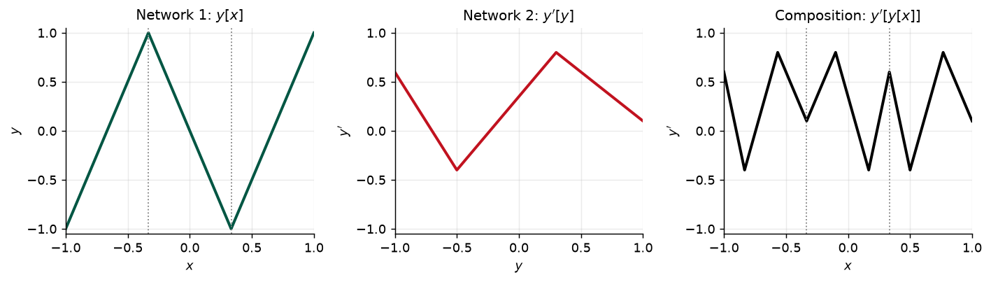
network 1 alone :  3 regions from 3 hidden units
network 2 alone :  3 regions from 3 hidden units
composition     :  9 regions from 6 hidden units
shallow, 6 units: at most 7Week 4 · Sessions 7–8 · September 15 & 17, 2026
A formative notebook spanning Weeks 3 and 4: joints, activation patterns, and slopes of a shallow network; counting regions and parameters; composition, folding, and clipping; the matrix form of a deep network; and what a trained network actually realizes. Every task ends in a self-check that tells you at once whether the idea landed.
In Colab choose File → Save a copy in Drive before you start. When you are done, Runtime → Run all, then File → Download → Download .ipynb and upload that file on Blackboard under Assignment A2, named A2_<lastname>.ipynb. The deadline is posted on Blackboard.
The answer key to the in-class multiple-choice review of Weeks 1–4, with the rationale for each answer and the section and page in Prince where the idea is covered.
Every section below opens with the section number and page range it covers in Prince, Understanding Deep Learning (MIT Press, 2024). Page numbers are those of the printed book. Figures taken from the textbook are captioned with their original figure number and page; figures generated by the code behind this page are ours. A complete cross-reference table appears in Section 11.
By the end of this week you should be able to:
This page shows the figures and results; the Python behind them is not printed here. All of it — every cell, in the order the note uses it — is in a notebook you can open in the browser with nothing to install:
Colab gives you a Python environment with NumPy, matplotlib, and PyTorch already installed. In Colab, run a cell with Shift+Enter. If you prefer to work locally, pip install -r requirements.txt from the course repository gives you the same environment.
Prince, Chapter 4 opening, p. 41.
Week 3 ended on a strong result and a weak one. The strong result was the universal approximation theorem: a shallow network with enough hidden units can describe any continuous function on a compact set to any precision. The weak result was everything the theorem leaves out. It says nothing about how many hidden units “enough” is, and for some functions the answer is impractically large.
This chapter introduces deep networks, which have more than one hidden layer. With ReLU activations they still compute continuous piecewise linear functions, exactly as shallow networks do, so nothing about the kind of function changes. What changes is the exchange rate. Prince’s claim for the chapter is that “deep networks can produce many more linear regions than shallow networks for a given number of parameters” (p. 41), and hence describe a broader family of functions in practice, if not in principle. The rest of the week makes that claim precise, then asks whether it is actually the reason deep networks work.
Prince §4.1, pp. 41–43; figures on pp. 42 and 44.
The cleanest way into deep networks is to take two shallow networks and feed the output of the first into the second (fig. 1a). Each has three hidden units. The first takes \(x\) and returns \(y\):
\[ y = \phi_0 + \phi_1 h_1 + \phi_2 h_2 + \phi_3 h_3. \tag{2}\]
The second takes \(y\) and returns \(y'\), with its own parameters, all primed:
\[ y' = \phi'_0 + \phi'_1 h'_1 + \phi'_2 h'_2 + \phi'_3 h'_3. \tag{4}\]
With ReLU activations the composition is still a piecewise linear function of \(x\). The question is how many pieces. A shallow network with six hidden units has at most seven regions. The composition, which also has six hidden units, can have more.
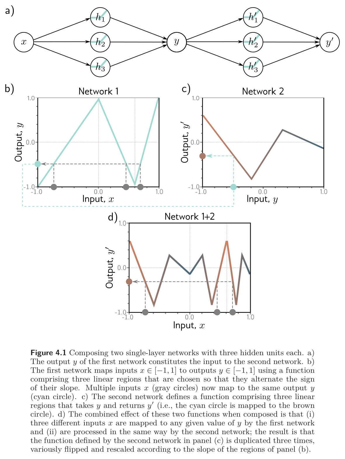
The mechanism is in fig. 1b–d. Choose the first network so that its three regions alternate in slope and each one sweeps the whole output range \(y \in [-1, 1]\). Then three different input ranges are mapped onto the same output range, and whatever the second network does to \(y \in [-1, 1]\) happens three times over as \(x\) runs from \(-1\) to \(1\), “variously flipped and rescaled according to the slope of the regions” (p. 42). The second network’s three regions are copied three times: nine linear regions from six hidden units.
Our version follows, with parameters chosen so that the counts can be checked. The first network is a zigzag with slopes \(3, -3, 3\) and joints at \(\pm 1/3\); the second is any three-region function on \([-1, 1]\). The region count is done by the method of Week 3: sample the input densely and count distinct activation patterns across all six hidden units, since every linear region of the composition has its own pattern.
network 1 alone : 3 regions from 3 hidden units
network 2 alone : 3 regions from 3 hidden units
composition : 9 regions from 6 hidden units
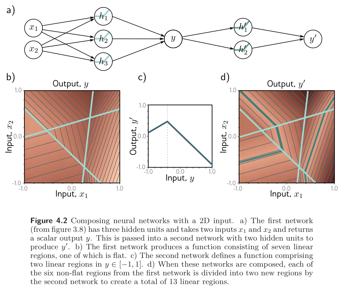
shallow, 6 units: at most 7The same principle applies in higher dimensions (fig. 3). There the first network is the two-input, three-unit network of Week 3, whose output surface has seven regions, one of them flat. Passing that through a second network with two regions splits each of the six non-flat regions in two, for thirteen in all. The flat region is not split, because a constant input gives the second network nothing to bend.
Prince §4.1, p. 43; figure on p. 44.
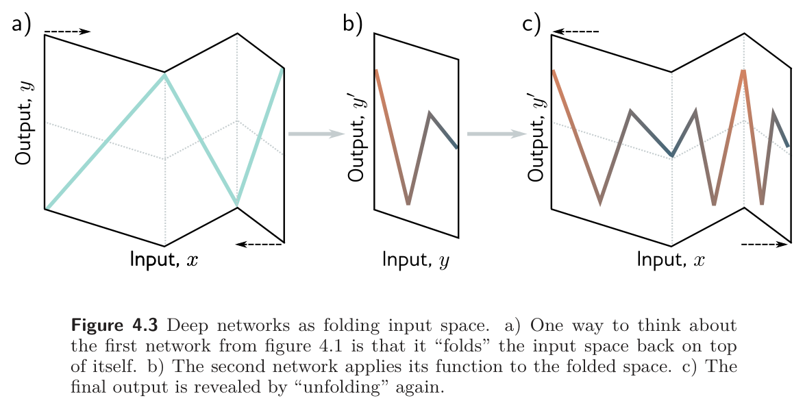
Prince offers a second picture of the same construction (fig. 4). The first network folds the input space back on itself, so that several inputs land on the same output. The second network then draws its function once on the folded paper. Unfolding reveals that function replicated at every point that had been stacked together, mirrored at each crease. The picture is worth keeping in mind for two reasons. It explains where the multiplication of regions comes from, and it exposes the price: the copies are not independent. The composition has nine regions but only twenty parameters, and the shapes of the nine pieces are tied to one another by the fold.
If one fold triples the regions, more folds should multiply them again. Fig. 5 composes the zigzag network with itself \(K\) times. Each composition adds three hidden units and, in the matrix notation of §4.4 below, twelve parameters. The regions go up by a factor of three each time.
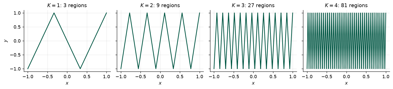
 layers K  hidden units  parameters  regions   3^K  shallow max
        1             3          10        3     3            4
        2             6          22        9     9            7
        3             9          34       27    27           10
        4            12          46       81    81           13
Twelve hidden units arranged as four layers of three make eighty-one regions. Twelve hidden units in a single layer make at most thirteen. That factor is the whole case for depth in one table, and the caveat that goes with it is in the figure: the eighty-one pieces are all the same triangle, at four scales. We return to this in §4.5.
Prince §4.2, pp. 43–45; figure on p. 45.
Composing two networks turns out to be a special case of something simpler. The output of the first network, eq. 2, is linear in the hidden units \(h_1, h_2, h_3\). The first thing the second network does to \(y\), inside the brackets of eq. 3, is also linear. A linear function of a linear function is linear, so substituting eq. 2 into eq. 3 gives
\[ \begin{aligned} h'_1 &= a[\theta'_{10} + \theta'_{11}y] = a[\theta'_{10} + \theta'_{11}\phi_0 + \theta'_{11}\phi_1 h_1 + \theta'_{11}\phi_2 h_2 + \theta'_{11}\phi_3 h_3] \\ h'_2 &= a[\theta'_{20} + \theta'_{21}y] = a[\theta'_{20} + \theta'_{21}\phi_0 + \theta'_{21}\phi_1 h_1 + \theta'_{21}\phi_2 h_2 + \theta'_{21}\phi_3 h_3] \\ h'_3 &= a[\theta'_{30} + \theta'_{31}y] = a[\theta'_{30} + \theta'_{31}\phi_0 + \theta'_{31}\phi_1 h_1 + \theta'_{31}\phi_2 h_2 + \theta'_{31}\phi_3 h_3], \end{aligned} \tag{5}\]
which, after renaming the constants, is
\[ \begin{aligned} h'_1 &= a[\psi_{10} + \psi_{11}h_1 + \psi_{12}h_2 + \psi_{13}h_3] \\ h'_2 &= a[\psi_{20} + \psi_{21}h_1 + \psi_{22}h_2 + \psi_{23}h_3] \\ h'_3 &= a[\psi_{30} + \psi_{31}h_1 + \psi_{32}h_2 + \psi_{33}h_3], \end{aligned} \tag{6}\]
with \(\psi_{10} = \theta'_{10} + \theta'_{11}\phi_0\), \(\psi_{11} = \theta'_{11}\phi_1\), \(\psi_{12} = \theta'_{11}\phi_2\), and so on. The intermediate variable \(y\) has disappeared. What is left is a network with two hidden layers, each of three units, in which every unit of the first layer feeds every unit of the second (fig. 6).
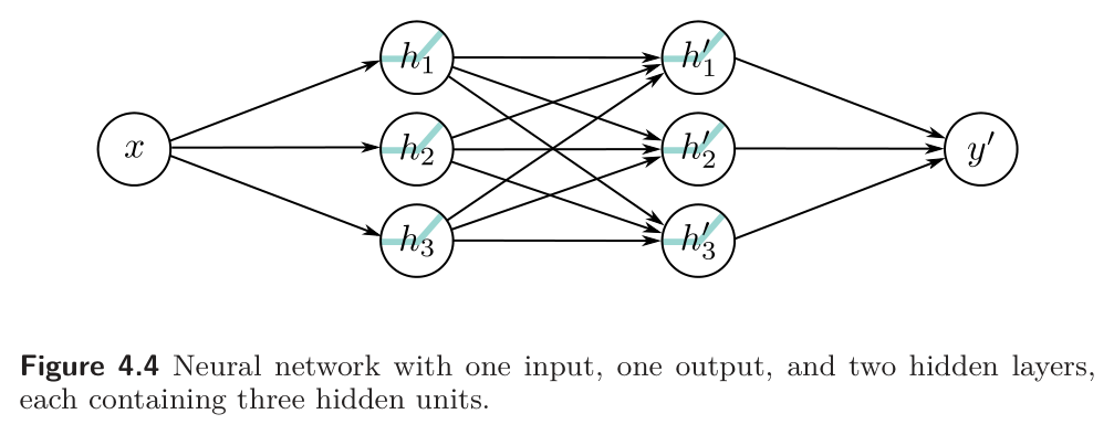
So a two-layer network can represent anything the composition can. It can also represent more. In eq. 6 the nine slopes \(\psi_{11}, \ldots, \psi_{33}\) are free, whereas in eq. 5 they are forced to be the outer product
\[ \boldsymbol{\Psi} = \begin{bmatrix} \theta'_{11} \\ \theta'_{21} \\ \theta'_{31} \end{bmatrix} \begin{bmatrix} \phi_1 & \phi_2 & \phi_3 \end{bmatrix}, \tag{7}\]
a \(3 \times 3\) matrix of rank one. The composition squeezes the three hidden units of the first layer through a single number \(y\) before the second layer sees them; the general two-layer network does not. We can check both halves of this claim, that the composition equals the two-layer network with the outer-product \(\boldsymbol{\Psi}\), and that this \(\boldsymbol{\Psi}\) is rank-deficient.
max |composition - two-layer network| = 2.2e-16
rank of the outer-product Psi = 1 (a free 3x3 Psi has rank up to 3)Prince §4.3, pp. 45–47; figure on p. 47.
Now take the general two-layer network of fig. 6 at face value. The first layer is
\[ h_1 = a[\theta_{10} + \theta_{11}x], \qquad h_2 = a[\theta_{20} + \theta_{21}x], \qquad h_3 = a[\theta_{30} + \theta_{31}x], \tag{8}\]
the second layer is eq. 6, which we restate as
\[ \begin{aligned} h'_1 &= a[\psi_{10} + \psi_{11}h_1 + \psi_{12}h_2 + \psi_{13}h_3] \\ h'_2 &= a[\psi_{20} + \psi_{21}h_1 + \psi_{22}h_2 + \psi_{23}h_3] \\ h'_3 &= a[\psi_{30} + \psi_{31}h_1 + \psi_{32}h_2 + \psi_{33}h_3], \end{aligned} \tag{9}\]
and the output is
\[ y' = \phi'_0 + \phi'_1 h'_1 + \phi'_2 h'_2 + \phi'_3 h'_3. \tag{10}\]
Reading these three equations in order gives a second picture of how depth builds complexity, this time in terms of clipping rather than folding (fig. 7):
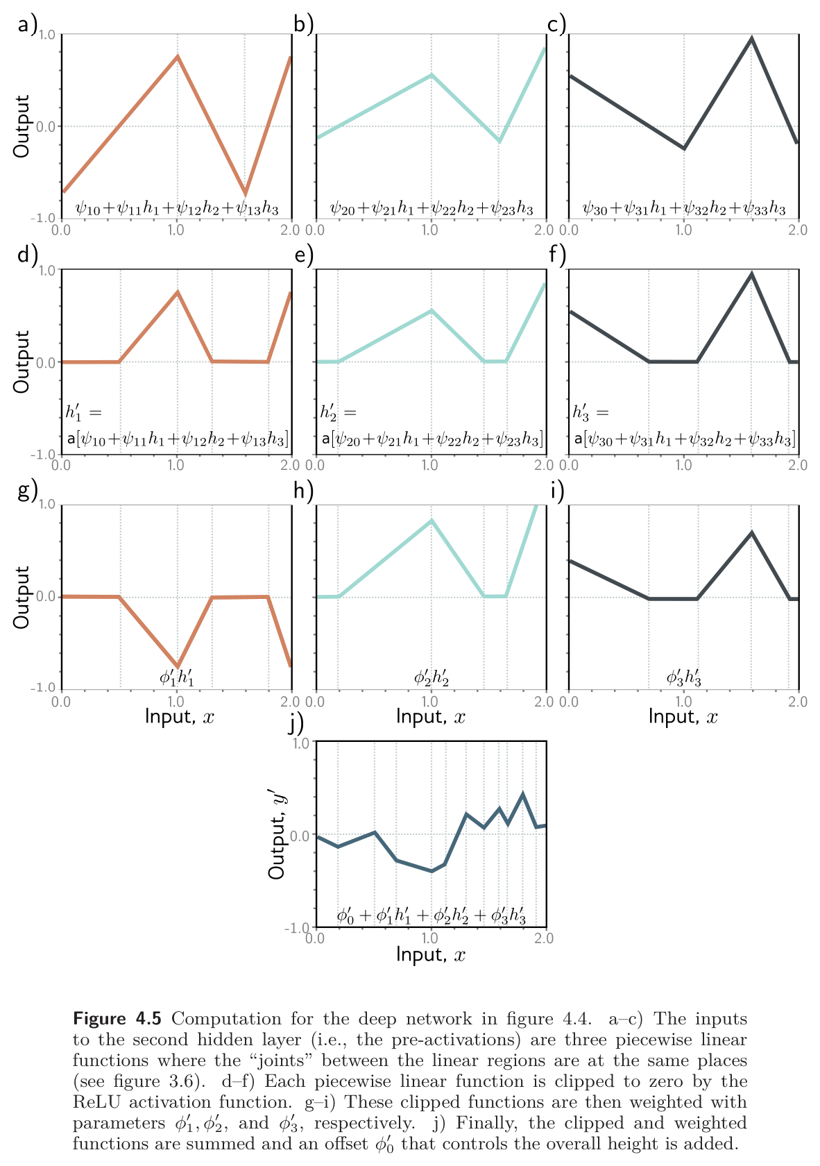
Fig. 8 is our version, with the first layer taken from Prince’s own figure 3.3 parameters (problem 3.8), so its three joints sit at \(x = 0.5\), \(1\), and \(1.57\) as they did last week. The second layer’s parameters are chosen so that each pre-activation crosses zero twice inside the plot. The code then counts the joints layer by layer.
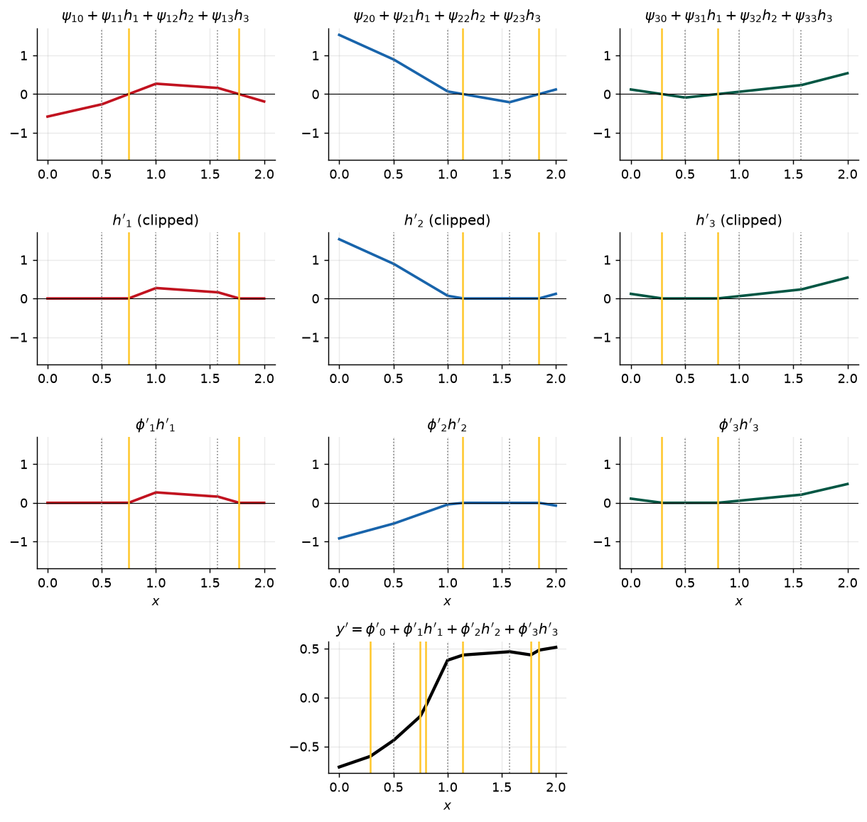
joints from layer 1            : 3
new joints added by layer 2    : 6  (2, 2, 2 per unit)
linear regions in the output   : 10  (= 1 + 3 + 6)
shallow network with 6 units   : at most 7
The joint count is the point. Six hidden units in one layer give at most six joints, and every joint is a zero-crossing of a line, so there is exactly one per unit. Six hidden units in two layers give three joints from the first layer plus as many from the second as its pre-activations can be made to cross zero, and those pre-activations are already piecewise linear, so each can cross several times. New joints multiply rather than add.
Folding and clipping describe the same computation. Folding shows the dependencies among the regions — the copies made by a fold are tied together — but hides how the new joints arise. Clipping shows the new joints but hides the dependencies. Prince is explicit that “both descriptions provide only partial insight into how deep neural networks operate” (p. 46), and that what we actually have is still just an equation from \(x\) to \(y'\). Written out in full by substituting eq. 8 into eq. 9 into eq. 10, it is
\[ \begin{aligned} y' = \phi'_0 &+ \phi'_1\, a\big[\psi_{10} + \psi_{11}a[\theta_{10} + \theta_{11}x] + \psi_{12}a[\theta_{20} + \theta_{21}x] + \psi_{13}a[\theta_{30} + \theta_{31}x]\big] \\ &+ \phi'_2\, a\big[\psi_{20} + \psi_{21}a[\theta_{10} + \theta_{11}x] + \psi_{22}a[\theta_{20} + \theta_{21}x] + \psi_{23}a[\theta_{30} + \theta_{31}x]\big] \\ &+ \phi'_3\, a\big[\psi_{30} + \psi_{31}a[\theta_{10} + \theta_{11}x] + \psi_{32}a[\theta_{20} + \theta_{21}x] + \psi_{33}a[\theta_{30} + \theta_{31}x]\big], \end{aligned} \tag{11}\]
“although this is admittedly rather difficult to understand” (p. 46). The matrix notation of the next section exists so that nobody has to write it.
Prince §4.3.1, p. 46.
Nothing stops us adding a third hidden layer, or a hundredth; modern networks may have more than a hundred layers with thousands of units in each. Three words fix the vocabulary. The number of hidden units in a layer is the network’s width, the number of hidden layers its depth, and the total number of hidden units is a measure of its capacity.
We write \(K\) for the number of hidden layers and \(D_1, D_2, \ldots, D_K\) for the number of units in each. These are hyperparameters: quantities chosen before the parameters (the slopes and intercepts) are learned. The distinction matters for how we think about a network. For fixed hyperparameters, say \(K = 2\) and \(D_1 = D_2 = 3\), the model is a family of functions and the parameters select one member. Letting the hyperparameters vary as well, a neural network is “a family of families of functions relating input to output” (p. 46). Chapter 8 takes up how to choose them.
Prince §4.4, pp. 48–49; figure on p. 48.
A deep network is linear transformations alternating with activation functions, and that structure is what matrix notation was built for (Appendix B.3; Week 2). Eq. 8, eq. 9, and eq. 10 become
\[ \begin{bmatrix} h_1 \\ h_2 \\ h_3 \end{bmatrix} = a\!\left[ \begin{bmatrix} \theta_{10} \\ \theta_{20} \\ \theta_{30} \end{bmatrix} + \begin{bmatrix} \theta_{11} \\ \theta_{21} \\ \theta_{31} \end{bmatrix} x \right], \qquad \begin{bmatrix} h'_1 \\ h'_2 \\ h'_3 \end{bmatrix} = a\!\left[ \begin{bmatrix} \psi_{10} \\ \psi_{20} \\ \psi_{30} \end{bmatrix} + \begin{bmatrix} \psi_{11} & \psi_{12} & \psi_{13} \\ \psi_{21} & \psi_{22} & \psi_{23} \\ \psi_{31} & \psi_{32} & \psi_{33} \end{bmatrix} \begin{bmatrix} h_1 \\ h_2 \\ h_3 \end{bmatrix} \right], \tag{12}\]
and \(y' = \phi'_0 + [\phi'_1 \;\; \phi'_2 \;\; \phi'_3]\,[h'_1 \;\; h'_2 \;\; h'_3]^T\), or more compactly
\[ \mathbf{h} = a[\boldsymbol{\theta}_0 + \boldsymbol{\theta}x], \qquad \mathbf{h}' = a[\boldsymbol{\psi}_0 + \boldsymbol{\Psi}\mathbf{h}], \qquad y' = \phi'_0 + \boldsymbol{\phi}'\mathbf{h}', \tag{13}\]
where \(a[\cdot]\) applies the activation function separately to every element of its vector argument.
Prince §4.4.1, pp. 48–49.
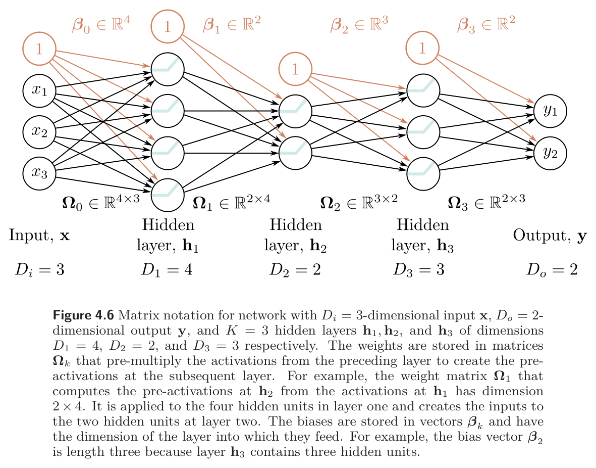
Primes and a fresh Greek letter per layer do not scale to a hundred layers. From here on the book, and this course, use one naming scheme for every layer. The vector of hidden units at layer \(k\) is \(\mathbf{h}_k\). The biases that feed layer \(k + 1\) are \(\boldsymbol{\beta}_k\), and the weights that act on layer \(k\) to produce the pre-activations of layer \(k + 1\) are \(\boldsymbol{\Omega}_k\). A deep network \(\mathbf{y} = \mathbf{f}[\mathbf{x}, \boldsymbol{\phi}]\) with \(K\) hidden layers is then
\[ \begin{aligned} \mathbf{h}_1 &= a[\boldsymbol{\beta}_0 + \boldsymbol{\Omega}_0\mathbf{x}] \\ \mathbf{h}_2 &= a[\boldsymbol{\beta}_1 + \boldsymbol{\Omega}_1\mathbf{h}_1] \\ \mathbf{h}_3 &= a[\boldsymbol{\beta}_2 + \boldsymbol{\Omega}_2\mathbf{h}_2] \\ &\;\;\vdots \\ \mathbf{h}_K &= a[\boldsymbol{\beta}_{K-1} + \boldsymbol{\Omega}_{K-1}\mathbf{h}_{K-1}] \\ \mathbf{y} &= \boldsymbol{\beta}_K + \boldsymbol{\Omega}_K\mathbf{h}_K, \end{aligned} \tag{14}\]
and the parameters are every one of these matrices and vectors, \(\boldsymbol{\phi} = \{\boldsymbol{\beta}_k, \boldsymbol{\Omega}_k\}_{k=0}^{K}\). Note that the output line has no activation function: the last step is purely linear, as it was for the shallow network.
The index on \(\boldsymbol{\beta}_k\) and \(\boldsymbol{\Omega}_k\) is the layer they are applied to, not the layer they produce: \(\boldsymbol{\Omega}_0\) acts on the input \(\mathbf{x}\) (layer zero) and \(\boldsymbol{\Omega}_K\) acts on the last hidden layer to produce \(\mathbf{y}\). A network with \(K\) hidden layers therefore has \(K + 1\) weight matrices and \(K + 1\) bias vectors.
Every size follows from where each object sits (fig. 9). If layer \(k\) has \(D_k\) hidden units, then the bias vector \(\boldsymbol{\beta}_{k-1}\) that feeds it has \(D_k\) entries, and the last bias vector \(\boldsymbol{\beta}_K\) has \(D_o\) entries, one per output. The first weight matrix \(\boldsymbol{\Omega}_0\) is \(D_1 \times D_i\), the last, \(\boldsymbol{\Omega}_K\), is \(D_o \times D_K\), and each one in between, \(\boldsymbol{\Omega}_k\), is \(D_{k+1} \times D_k\): rows for the layer it produces, columns for the layer it consumes.
Finally, the whole network can be written as one nested expression,
\[ \mathbf{y} = \boldsymbol{\beta}_K + \boldsymbol{\Omega}_K\, a\Big[\boldsymbol{\beta}_{K-1} + \boldsymbol{\Omega}_{K-1}\, a\big[\ldots\, \boldsymbol{\beta}_2 + \boldsymbol{\Omega}_2\, a[\boldsymbol{\beta}_1 + \boldsymbol{\Omega}_1\, a[\boldsymbol{\beta}_0 + \boldsymbol{\Omega}_0\mathbf{x}]]\ldots\big]\Big], \tag{15}\]
which is eq. 11 with the subscripts tidied up, and no easier to read. In PyTorch, though, it is one line. A Linear layer is \(\boldsymbol{\beta}_k +
\boldsymbol{\Omega}_k \mathbf{h}_k\), and its weight and bias attributes are the matrix and vector exactly, with the shapes just described. The following builds the network of fig. 9 and prints every shape, which is the check problem 4.2 asks for.
layer      Omega_k shape  beta_k size   reads
k = 0             (4, 3)            4   h_1 = a[beta_0 + Omega_0 x]
k = 1             (2, 4)            2   h_2 = a[beta_1 + Omega_1 h_1]
k = 2             (3, 2)            3   h_3 = a[beta_2 + Omega_2 h_2]
k = 3             (2, 3)            2   y = beta_3 + Omega_3 h_3

total parameters: 43
Row counts match the layer each matrix produces and column counts the layer it consumes, as the figure says: \(\boldsymbol{\Omega}_1\) is \(2 \times 4\) because it turns four units into two. Summing entries gives the parameter count, which for the general case with \(D_i\) inputs, \(D_o\) outputs, and widths \(D_1, \ldots, D_K\) is
\[ \underbrace{D_1(D_i + 1)}_{\boldsymbol{\Omega}_0,\, \boldsymbol{\beta}_0} + \sum_{k=1}^{K-1} \underbrace{D_{k+1}(D_k + 1)}_{\boldsymbol{\Omega}_k,\, \boldsymbol{\beta}_k} + \underbrace{D_o(D_K + 1)}_{\boldsymbol{\Omega}_K,\, \boldsymbol{\beta}_K}. \tag{16}\]
Prince §4.5, pp. 49–51; figure on p. 51.
Week 3 described shallow networks and this week deep ones. Prince compares them along five lines, and it is worth being clear about which comparisons are theorems, which are counting arguments, and which are observations.
Prince §4.5.1, p. 50.
Both can approximate any continuous function. The shallow case is the universal approximation theorem of Week 3. The deep case follows from it: a two-layer network contains the composition of two shallow networks as a special case, and if the second of those computes the identity function (problem 4.7), the deep network is a shallow network. So a deep network with enough capacity can approximate any continuous function arbitrarily closely. This is a theorem, and by itself it says nothing about which architecture is better.
Prince §4.5.2, p. 50; notes on pp. 52–53.
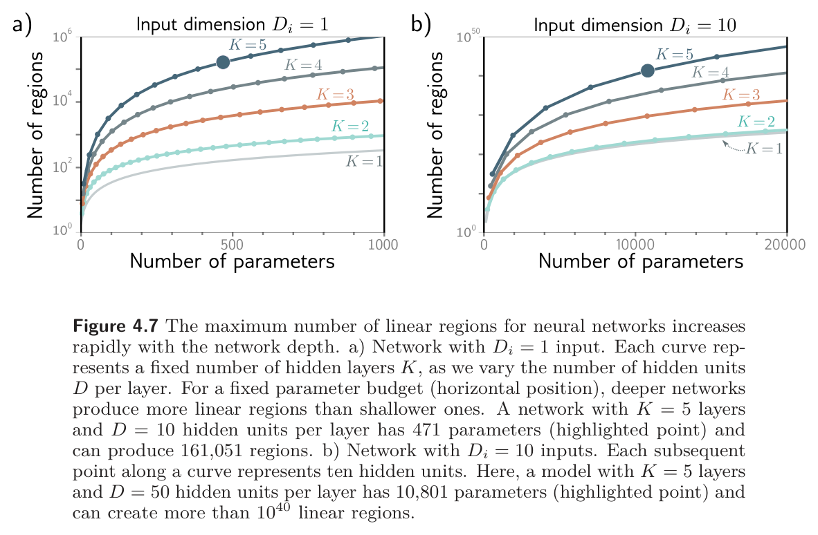
Here the two differ. For one input and one output, a shallow network with \(D > 2\) hidden units makes at most \(D + 1\) linear regions from \(3D + 1\) parameters. A deep network with \(K\) layers of \(D > 2\) units each makes up to
\[ (D + 1)^K \;\text{ regions from }\; 3D + 1 + (K - 1)D(D + 1) \;\text{ parameters}. \tag{17}\]
Regions grow exponentially in depth; parameters grow only linearly. The parameter count is eq. 16 with \(D_i = D_o = 1\) and every width equal to \(D\) (problem 4.10), and the region count is the folding argument of §4.1 done \(K\) times: each layer can fold the input into \(D + 1\) pieces on which the next layer’s function is replicated, just as fig. 5 folded it into three. Fig. 10a plots regions against parameters for depths one to five, and the gap widens with every layer. The book’s headline example is a network with \(K = 5\) and \(D = 10\): 471 parameters and 161,051 regions.
With more inputs the maximum is harder to compute, but the chapter notes (p. 53) give a closed form for the case where every layer has the same width \(D\) and \(D\) is a multiple of \(D_i\):
\[ N_r = \left(\frac{D}{D_i} + 1\right)^{D_i(K-1)} \sum_{j=0}^{D_i} \binom{D}{j}. \tag{18}\]
The first factor is the first \(K - 1\) layers folding the space, with \(D / D_i\) units now needed per input dimension to make each fold. The sum is the Zaslavsky bound of Week 3, the regions the final layer carves out of each folded piece. Fig. 11 evaluates both formulas and reproduces the two points the book highlights.
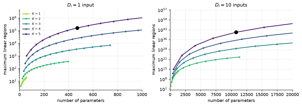
K = 5, D = 10, D_i = 1 :    471 parameters,    161,051 regions
K = 5, D = 50, D_i = 10: 10,801 parameters, about 10^41 regionsThis is the place to be careful. A deep network’s regions “contain complex dependencies and symmetries” (p. 50): the folding picture showed that the copies are mirror images of one another, and fig. 5 was eighty-one regions made of one triangle. The flexibility of the function is still bounded by the number of parameters, and forty-six parameters cannot describe eighty-one independent pieces. Prince’s conclusion is conditional: the extra regions are an advantage only if (i) the function we want to approximate has similar symmetries, or (ii) we have reason to believe the mapping from input to output “really does involve a composition of simpler functions” (p. 51). For many engineering systems (ii) is a reasonable belief, and it is a better argument for depth than the raw count is.
Prince §4.5.3, p. 50; notes on p. 53.
There is a stronger theoretical statement than region counting. For certain functions, a shallow network needs exponentially more hidden units than a deep network to reach the same approximation error. This is the depth efficiency of neural networks, and the chapter notes trace it through Telgarsky (2016), who builds one-input functions realizable with \(O[k^3]\) layers of constant width that no network of \(O[k]\) layers and width below \(2^k\) can match, and Eldan & Shamir (2016), who show that with multivariate inputs some three-layer networks cannot be realized by any two-layer network of sub-exponential size. The corresponding width efficiency results (Lu et al., 2017) are weaker: a wide shallow network needs at most a polynomial increase in depth to be matched by a narrow one. Depth is the more valuable resource. The same caveat applies as before, though: it is not clear that the functions we meet in practice belong to the classes these theorems describe.
Prince §4.5.4, pp. 50–51.
Everything so far has been fully connected: every unit in one layer feeds every unit in the next. For an image with a million pixels that is not practical, and the reason is not only the parameter count. We want different parts of the image to be processed the same way, because there is no point learning to recognize an object separately at every position it might appear. The solution is to process local regions in parallel and then integrate information from progressively larger regions. Such local-to-global processing is hard to specify without multiple layers, and it is the subject of Chapter 10.
fully connected first layer,   100 hidden units:    300,000,100 parameters  (  1.2 GB in float32)
fully connected first layer,  1000 hidden units:  3,000,001,000 parameters  ( 12.0 GB in float32)
One layer of a thousand units, on one photograph, already needs twelve gigabytes of weights, and every one of those weights would have to be learned from data. The count is the least of the problems; the missing structure is the real one.
Prince §4.5.5, p. 51.
The last two comparisons are empirical. Moderately deep networks are usually easier to fit than shallow ones, perhaps because over-parameterized deep models have a large family of roughly equivalent solutions that are easy to find. Past a certain depth, training becomes difficult again, and much of Chapter 11 is about the methods that mitigate this. Deep networks also seem to generalize better to new data. In practice the best results on most tasks come from networks with tens or hundreds of layers, and “neither of these phenomena are well understood” (p. 51); Chapter 20 returns to both.
Ours; UDL notebook 4.3.
The theory of §4.5 is about what a network can represent. Whether gradient descent finds it is a different question, and Chapters 6 and 7 are about the answer. We can preview the gap now. Problem 4.11 poses two networks with the same parameter count: a shallow one with \(D = 95\) hidden units and a deep one with \(K = 10\) layers of \(D = 5\). By eq. 17 the shallow network can make 96 regions and the deep one about sixty million. We fit both, with the Adam optimizer of Week 2, to noisy samples of a triangle wave, a target whose repeated symmetric pieces are exactly the kind of structure a fold reproduces for free. Then we count the regions each trained network actually uses, by tallying activation patterns across every hidden unit, as in fig. 2.
network                parameters  max regions  realized  final MSE
shallow, D = 95               286           96        34     0.0023
deep, K = 10, D = 5           286   60,466,176        20     0.3227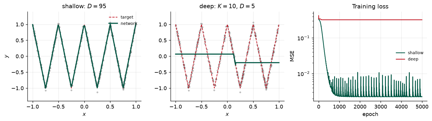
Two things stand out. Neither network comes anywhere near its maximum region count: the shallow one realizes about half of its 96, and the deep one a couple of dozen of its sixty million. And on this target, with this optimizer and this much training, the shallow network wins outright. The maximum in eq. 17 is a statement about the best parameter setting; gradient descent from a random start does not find it, and for a narrow, deep ReLU network it barely gets started, for reasons Chapter 7 will make precise when we look at how gradients propagate through many layers. Meanwhile the hand-built network of fig. 5, with forty-six parameters, would fit a triangle wave exactly. The capacity is real. Reaching it is the hard part, and it is why the remainder of the course is mostly about training.
Prince §4.6, p. 52.
Composing two shallow networks makes the first network fold the input space and the second apply a piecewise linear function that is duplicated wherever the space was folded onto itself. That composition is a special case of a network with two hidden layers, in which the second-layer ReLUs clip the incoming functions and add joints. Hyperparameters — the depth \(K\) and the widths \(D_1, \ldots, D_K\) — fix the family; parameters \(\{\boldsymbol{\beta}_k, \boldsymbol{\Omega}_k\}\) fix the member, and the general network is \(K + 1\) affine maps with a ReLU between each pair, eq. 14.
Comparing shallow with deep: (i) both approximate any continuous function given enough capacity; (ii) deep networks produce many more linear regions per parameter, though the regions are tied together by the folds; (iii) some functions need exponentially more shallow units than deep ones; (iv) large, structured inputs like images are best handled in stages, which needs layers; and (v) in practice the best results come from deep networks with many layers, for reasons that are not yet understood.
Next: we now know what shallow and deep networks can represent, and we have seen that representing a function and finding it are different problems. Chapter 5 introduces loss functions, which turn “how wrong is this model” into a single number for any choice of parameters. Chapters 6 and 7 then describe the search for the parameters that minimize it.
1. (UDL 4.1*) Consider composing the two networks in fig. 13. Sketch the relationship between \(x\) and \(y'\) for \(x \in [-1, 1]\). How many linear regions does it have, and how does that follow from the number of regions in panels (b) and (c)? Then check your sketch in the notebook by encoding both panels as shallow networks and composing them as fig. 2 does.
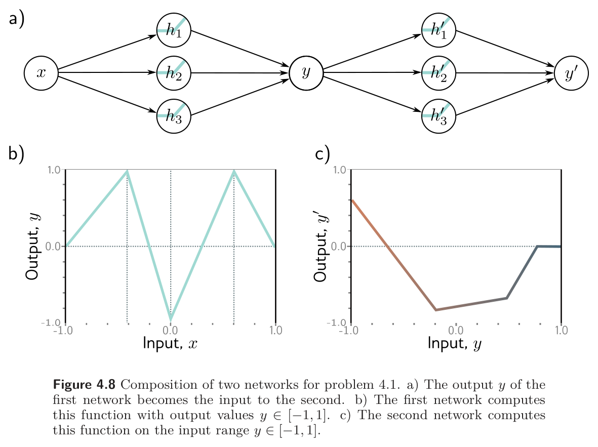
2. (UDL 4.2, 4.5, and 4.6) Identify the four hyperparameters in fig. 9. For a network with \(D_i = 5\) inputs, \(D_o = 1\) output, and \(K = 20\) hidden layers of \(D = 30\) units each, state the depth and the width. Then consider a network with \(D_i = D_o = 1\) and \(K = 10\) layers of \(D = 10\) units: would the number of weights increase more if the depth grew by one or if the width grew by one? Show your reasoning using eq. 16.
3. (UDL 4.3) Use the non-negative homogeneity of the ReLU (problem 3.5) to show that for non-negative scalars \(\lambda_0, \lambda_1\), \[ \mathrm{ReLU}\big[\boldsymbol{\beta}_1 + \lambda_1 \boldsymbol{\Omega}_1 \mathrm{ReLU}[\boldsymbol{\beta}_0 + \lambda_0 \boldsymbol{\Omega}_0 \mathbf{x}]\big] = \lambda_0 \lambda_1 \mathrm{ReLU}\Big[\tfrac{1}{\lambda_0\lambda_1}\boldsymbol{\beta}_1 + \boldsymbol{\Omega}_1 \mathrm{ReLU}\big[\tfrac{1}{\lambda_0}\boldsymbol{\beta}_0 + \boldsymbol{\Omega}_0 \mathbf{x}\big]\Big]. \] Explain in one sentence what this says about the uniqueness of a trained network’s weights, and connect it to your answer to problem 4 of Week 3.
4. (UDL 4.4) Write out the equations for a network with \(D_i = 5\) inputs, \(D_o = 4\) outputs, and three hidden layers of sizes \(D_1 = 20\), \(D_2 = 10\), and \(D_3 = 7\), in both the layered form of eq. 14 and the nested form of eq. 15. Give the size of every \(\boldsymbol{\Omega}_k\) and \(\boldsymbol{\beta}_k\), and the total parameter count from eq. 16. Then build it with make_mlp in the notebook and confirm every size.
5. (UDL 4.7) Choose parameters for the ten-parameter shallow network of Week 3 so that it computes the identity function \(y = x\) over a finite range \(x \in [a, b]\). Hence explain why the argument of §4.5.1 — that a deep network can approximate any continuous function — is a consequence of the shallow result rather than a new theorem.
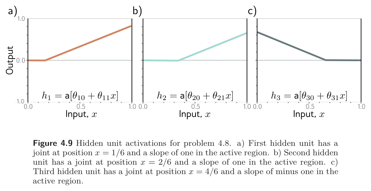
6. (UDL 4.8* and 4.9*) Fig. 14 shows three hidden-unit activations with slopes \(1, 1, -1\) and joints at \(x = 1/6\), \(2/6\), and \(4/6\). Find \(\phi_0, \phi_1, \phi_2, \phi_3\) such that \(\phi_0 + \phi_1 h_1 + \phi_2 h_2 + \phi_3 h_3\) has four linear regions oscillating between output values zero and one, with the leftmost slope positive. How many regions result if this network is composed with itself? Composed with itself \(K\) times? Then decide whether the same kind of oscillation with three regions is possible using two hidden units, and with five regions using four, and explain the pattern.
7. (UDL 4.10 and 4.11*) Show that a network with one input, one output, and \(K\) hidden layers of \(D\) units has \(3D + 1 + (K - 1)D(D + 1)\) parameters. Then compare the two networks of the PyTorch section: shallow with \(D = 95\), and deep with \(K = 10\), \(D = 5\). Confirm both have 286 parameters, compute the maximum regions for each, and argue which would run faster at inference time. Is the region count the right basis for choosing between them? Use the printed results of the shallow-vs-deep cell in your answer.
8. A laser powder-bed fusion machine records a \(256 \times 256\) thermal image of the melt pool at each scan step, and a quality model must predict the porosity of the finished part from it. (a) Count the parameters of a fully connected first layer with \(D_1 = 512\) hidden units, and comment in the light of §4.5.4. (b) A process engineer describes the physics as a chain: laser parameters set the melt-pool geometry, geometry sets the local cooling rate, cooling rate sets the microstructure, and microstructure sets the porosity. Explain, citing §4.5.2 and the folding picture, why this description is an argument for a deep model rather than a wide one, and write down the hyperparameters of a network whose layers mirror the chain.
9. Computational. The deep network in the PyTorch section is unusually narrow. In the notebook, refit with \(K = 3\) layers of \(D = 8\) units (169 parameters) and with \(K = 2\) layers of \(D = 12\), from three different random seeds each. Tabulate final MSE and realized regions for every run. Which configuration is most sensitive to the seed, and what does that suggest about the loss surface that Chapter 6 will have to navigate?
10. Computational. In fig. 5 the region count triples per layer because every region of the zigzag sweeps the full output range \([-1, 1]\). Rescale the first network’s output by \(0.5\) (halve \(\phi_0\) and every \(\phi_d\)) and repeat the composition for \(K = 1, \ldots, 4\). Count the regions, explain why the count now falls short of \(3^K\), and relate this to the word “up to” in eq. 17.
Every part of this page, mapped to Prince, Understanding Deep Learning (MIT Press, 2024) (Prince 2024). Page numbers are those of the printed book.
| This page | Prince section | Pages | Figures used |
|---|---|---|---|
| Why Go Deep | Ch. 4 opening | 41 | — |
| Composing Two Networks | §4.1 | 41–43 | 4.1 (p. 42), 4.2 (p. 44) |
| — Folding the input space | §4.1 | 43 | 4.3 (p. 44) |
| From Composition to a Deep Network | §4.2 | 43–45 | 4.4 (p. 45) |
| Deep Neural Networks | §4.3 | 45–46 | 4.5 (p. 47) |
| — Hyperparameters | §4.3.1 | 46 | — |
| Matrix Notation | §4.4 | 48–49 | — |
| — The general formulation | §4.4.1 | 48–49 | 4.6 (p. 48) |
| Shallow vs. Deep Networks | §4.5 | 49 | — |
| — Approximation power | §4.5.1 | 50 | — |
| — Linear regions per parameter | §4.5.2 and Notes | 50, 52–53 | 4.7 (p. 51) |
| — Depth efficiency | §4.5.3 and Notes | 50, 53 | — |
| — Large, structured inputs | §4.5.4 | 50–51 | — |
| — Training and generalization | §4.5.5 | 51 | — |
| Deep Networks in PyTorch | ours; notebook 4.3 | — | — |
| Summary | §4.6 | 52 | — |
| Exercises 1–7 | Problems 4.1–4.11 | 53–55 | 4.8 (p. 54), 4.9 (p. 55) |
Equations on this page correspond to Prince as follows: eq. 1 is his (4.1), eq. 2 is (4.2), eq. 3 is (4.3), eq. 4 is (4.4), eq. 5 is (4.5), eq. 6 is (4.6), eq. 8 is (4.7), eq. 9 is (4.8), eq. 10 is (4.9), eq. 11 is (4.10), eq. 12 collects (4.11)–(4.13), eq. 13 is (4.14), eq. 14 is (4.15), eq. 15 is (4.16), and eq. 18 is (4.17) from the chapter notes. Eq. 7 is the outer-product constraint stated in prose on p. 45, eq. 17 is the region and parameter count stated in prose in §4.5.2, and eq. 16 is the general parameter count implied by §4.4.1; none of these three appears as a numbered equation in the book.
Figures 4.1–4.9 are reproduced unaltered from Prince, Understanding Deep Learning (MIT Press, 2024), which is distributed under a Creative Commons CC-BY-NC-ND license, and are used here for non-commercial classroom instruction. All other figures on this page are generated by the code in this week’s notebook.