x: shape (3,), ndim 1, 3 numbers
Y: shape (2, 3), ndim 2, 6 numbers
Z: shape (2, 3, 4), ndim 3, 24 numbers

torch types: Tensor Tensor Tensor
torch shapes: (3,) (2, 3) (2, 3, 4)Mathematical and Computational Background
Week 2 · Sessions 3–4 · September 1 & 3, 2026
foundations
The linear algebra and matrix calculus of Appendix B, written as runnable Python, and supervised learning revisited as a family of functions with a loss.
How to read the references in these notes
Every section opens with the section it covers in Prince, Understanding Deep Learning (MIT Press, 2024). Chapter references carry printed page numbers; Appendix B is cited by section number. Figures taken from the textbook are captioned with their original figure number; figures generated for this note are ours. A complete cross-reference table appears in Section 11.
1 Learning Objectives
By the end of this week you should be able to:
- Read and write the book’s vector, matrix, and tensor notation, and build each object in both NumPy and PyTorch.
- Compute transposes, norms, matrix products, dot products, and inverses, and say what each one costs.
- Explain what the eigenspectrum, determinant, and trace tell you about the geometry of a linear map.
- Recognize diagonal, triangular, orthogonal, and permutation matrices, and exploit the shortcut each one offers.
- Write a system of linear equations as \(\mathbf{y} = \boldsymbol{\phi}_0 + \boldsymbol{\Phi}\mathbf{z}\), and find that same form inside a PyTorch layer.
- State the shape of \(\partial \mathbf{y} / \partial \mathbf{x}\) for scalar, vector, and matrix arguments, and obtain it with automatic differentiation.
- Restate supervised learning as picking one member of a family \(\mathbf{f}[\mathbf{x}, \boldsymbol{\phi}]\), define the least-squares loss, and train 1D linear regression three different ways.
- Explain, using the eigenspectrum of the loss surface, why rescaling an input changes how fast gradient descent converges.
The code lives in a notebook
This page shows the figures and results; the Python behind them is not printed here. All of it — every cell, in the order the note uses it — is in a notebook you can open in the browser with nothing to install:
- ▶ Open the Week 2 notebook in Google Colab — all of this page’s code, in order.
- ▶ UDL notebook 1.1 — Background mathematics — Prince’s own exercises on linear functions, derivatives, and sums.
- ▶ UDL notebook 2.1 — Supervised learning — the 1D linear regression fit of §2.2, by hand.
Colab gives you a Python environment with NumPy, matplotlib, and PyTorch already installed. In Colab, run a cell with Shift+Enter; !pip install anything else you need. If you prefer to work locally, pip install -r requirements.txt from the course repository gives you the same environment.
Assignment A1 — Foundations
A formative notebook spanning Weeks 1 and 2: the learning paradigms, the supervised recipe, and the Appendix B algebra behind one layer. Every task ends in a self-check that tells you at once whether the idea landed.
- ▶ Open A1 in Google Colab — nothing to install.
In Colab choose File → Save a copy in Drive before you start. When you are done, Runtime → Run all, then File → Download → Download .ipynb and upload that file on Blackboard under Assignment A1, named A1_<lastname>.ipynb. The deadline is posted on Blackboard.
2 Why an Appendix Gets a Whole Week
Prince puts the mathematics in an appendix because the book is about ideas, not about linear algebra. We spend a week on it anyway, for a practical reason: from Chapter 3 onward, every model in this course is a stack of the object in eq. 12 with a nonlinearity dropped between the layers. If \(\boldsymbol{\Phi}\mathbf{z}\) and \(\partial \mathbf{y}/\partial \mathbf{x}\) are comfortable, the rest of the semester is about which \(\boldsymbol{\Phi}\) and how to find it. If they are not, every chapter will feel like notation.
So this note takes Appendix B one section at a time and writes each definition as code you can run. Then it returns to Chapter 2 and does supervised learning again, this time with the matrix machinery in hand.
3 Vectors, Matrices, and Tensors
Prince §B.3.
A vector \(\mathbf{x} \in \mathbb{R}^{D}\) is a one-dimensional array of \(D\) numbers, which we always take to be arranged in a column. A matrix \(\mathbf{Y} \in \mathbb{R}^{D_1 \times D_2}\) is a two-dimensional array with \(D_1\) rows and \(D_2\) columns. A tensor \(\mathbf{z} \in \mathbb{R}^{D_1 \times D_2 \dots \times D_N}\) is an \(N\)-dimensional array.
Prince flags the terminological trap himself: all three of these are stored in objects called “tensors” in PyTorch and TensorFlow. In this course, tensor means whichever of the three the shape says it is, and the shape is the thing to check first when code misbehaves.
Notation
Prince writes function application with square brackets, \(f[\cdot]\), reserving parentheses for grouping. Vectors are bold lowercase, matrices bold uppercase, and scalars plain. Parameters are collected in \(\boldsymbol{\phi}\). We follow that convention everywhere, including in variable names in the code.
A column vector is a matrix with one column, but NumPy’s one-dimensional arrays are neither rows nor columns until you say so. That ambiguity is the single most common source of shape bugs in student code, so it is worth being deliberate:
1-D array      : (3,) -- neither row nor column
explicit column: (3, 1)
explicit row   : (1, 3)

column - row gives an outer difference:
[[ 0. -1. -2.]
 [ 1.  0. -1.]
 [ 2.  1.  0.]]
3.1 Transpose
Prince §B.3.1.
The transpose \(\mathbf{A}^T \in \mathbb{R}^{D_2 \times D_1}\) of a matrix \(\mathbf{A} \in \mathbb{R}^{D_1 \times D_2}\) reflects it about the principal diagonal, so the \(k^{th}\) column becomes the \(k^{th}\) row. Transposing a product reverses the order:
\[ (\mathbf{A}\mathbf{B})^T = \mathbf{B}^T \mathbf{A}^T. \tag{1}\]
The transpose of a column vector is a row vector and vice versa. Checking eq. 1 on a random product:
A: (3, 4)  B: (4, 2)  AB: (3, 2)  (AB)^T: (2, 3)
(AB)^T == B^T A^T : True
A^T B^T is not even defined: (4, 3) x (2, 4)
The order reversal is not a convention you have to remember; it is forced by the shapes. \(\mathbf{A}^T\mathbf{B}^T\) would ask a \(4 \times 3\) matrix to multiply a \(2 \times 4\) one, which is not a legal product.
3.2 Vector and matrix norms
Prince §B.3.2.
For a vector \(\mathbf{z}\), the \(\ell_p\) norm is
\[ \lVert \mathbf{z} \rVert_p = \left( \sum_{d=1}^{D} \lvert z_d \rvert^{p} \right)^{1/p}. \tag{2}\]
When \(p = 2\) this is the length of the vector — the Euclidean norm, which is so much the default in deep learning that the subscript is usually dropped and it is written \(\lVert \mathbf{z} \rVert\). When \(p = \infty\) the operator returns the largest absolute entry. The same idea extends to matrices: the \(\ell_2\) norm of a matrix \(\mathbf{Z}\) is the Frobenius norm,
\[ \lVert \mathbf{Z} \rVert_F = \left( \sum_{i=1}^{I} \sum_{j=1}^{J} \lvert z_{ij} \rvert^{2} \right)^{1/2}, \tag{3}\]
which is just the Euclidean norm of the matrix flattened into one long vector. The three vector norms of \(\mathbf{z} = [3, -4, 12]^T\), and the two readings of the Frobenius norm:
||z||_1    = 19.0000
||z||_2    = 13.0000
||z||_inf  = 12.0000

||Z||_F              = 5.4772
Euclidean norm of the flattened matrix = 5.4772
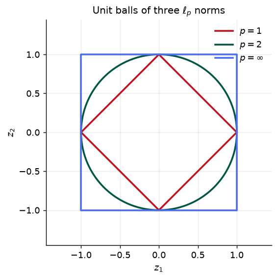
Which \(p\) you choose changes what “small” means, and that has consequences we will meet again in Chapter 9, where a norm added to the loss is what regularization is. fig. 1 shows the shape of the set of vectors whose norm equals one under each choice.
3.3 Products
Prince §B.3.3–§B.3.4.
The product \(\mathbf{C} = \mathbf{A}\mathbf{B}\) of matrices \(\mathbf{A} \in \mathbb{R}^{D_1 \times D_2}\) and \(\mathbf{B} \in \mathbb{R}^{D_2 \times D_3}\) is the matrix \(\mathbf{C} \in \mathbb{R}^{D_1 \times D_3}\) with entries
\[ C_{ij} = \sum_{d=1}^{D_2} A_{id} B_{dj}. \tag{4}\]
The dot product of two vectors \(\mathbf{a}, \mathbf{b} \in \mathbb{R}^{D}\) is the scalar
\[ \mathbf{a}^T \mathbf{b} = \mathbf{b}^T \mathbf{a} = \sum_{d=1}^{D} a_d b_d, \tag{5}\]
and it is proportional to the two lengths and the cosine of the angle \(\theta\) between the vectors:
\[ \mathbf{a}^T \mathbf{b} = \lVert \mathbf{a} \rVert \, \lVert \mathbf{b} \rVert \cos[\theta]. \tag{6}\]
eq. 6 is worth committing to memory. It is why a dot product is the natural way to ask “how aligned are these two things?”, and it is the operation at the heart of the attention mechanism in Chapter 12. Written out as a loop, eq. 4 reproduces what the @ operator does, and eq. 6 recovers the angle between two vectors:
(B.10) as an explicit loop matches the @ operator: True

a . b            = 5.0000
||a|| ||b|| cos t = 5.0000
angle between them = 47.61 degrees
3.4 Inverse
Prince §B.3.5.
A square matrix \(\mathbf{A}\) may or may not have an inverse \(\mathbf{A}^{-1}\) with \(\mathbf{A}^{-1}\mathbf{A} = \mathbf{A}\mathbf{A}^{-1} = \mathbf{I}\). A matrix with no inverse is singular. Inverses of products, like transposes, reverse:
\[ (\mathbf{A}\mathbf{B})^{-1} = \mathbf{B}^{-1} \mathbf{A}^{-1}. \tag{7}\]
Inverting a \(D \times D\) matrix in general takes \(\mathcal{O}[D^3]\) operations, which is the reason so much of numerical linear algebra is about avoiding it.
(MN)^-1 == N^-1 M^-1 : True
det(S) = 0.0  -> singular, no inverse

Cost of a D x D inverse, in units of elementary operations:
      D                D^3     relative to D=10
     10              1,000                    1x
    100          1,000,000                1,000x
   1000      1,000,000,000            1,000,000x
  10000  1,000,000,000,000        1,000,000,000x
Ten thousand inputs is a small image, and a dense \(10{,}000 \times 10{,}000\) inverse is a trillion operations. This is why we will never invert anything in this course: we will solve, factorize, or — from Chapter 6 onward — walk downhill instead.
3.5 Subspaces
Prince §B.3.6.
Consider \(\mathbf{A} \in \mathbb{R}^{D_1 \times D_2}\). The product \(\mathbf{A}\mathbf{x}\) is the \(D_2\) columns of \(\mathbf{A}\) weighted by the \(D_2\) entries of \(\mathbf{x}\), so the set of reachable outputs is exactly the linear subspace spanned by the columns — the column space. The part of the input space that gets crushed to nothing, \(\{\mathbf{x} : \mathbf{A}\mathbf{x} = \mathbf{0}\}\), is the nullspace.
Read the inequality in §B.3.6 carefully
The passage says the product cannot reach the whole output space when there are more columns than rows. The sentence that follows it — and the geometry — give the correct condition: \(\mathbf{A}\mathbf{x}\) reaches only the span of the columns, so it fails to fill \(\mathbb{R}^{D_1}\) when the column space has dimension less than \(D_1\), which for a full-rank matrix means \(D_2 < D_1\): a tall, “portrait” matrix. A wide matrix (\(D_2 > D_1\)) covers the output space but pays for it with a nullspace of dimension at least \(D_2 - D_1\). The output below checks both cases.
tall (3x2): rank 2, column space is 2-D inside R^3, nullspace is 0-D inside R^2
wide (2x3): rank 2, column space is 2-D inside R^2, nullspace is 1-D inside R^3

residuals of x1 + x2 - x3 for five random outputs: [0. 0. 0. 0. 0.]
wide @ nullspace direction = [0. 0.]
3.6 Eigenspectrum, determinant, and trace
Prince §B.3.7–§B.3.8.
Multiply every point on the unit circle by a \(2 \times 2\) matrix and the circle becomes an ellipse, as in fig. 2. The radii of the major and minor axes record how much the transformation stretches space in its most and least expanded directions. In higher dimensions a \(D\)-dimensional sphere maps to a \(D\)-dimensional ellipsoid and the same reading applies.
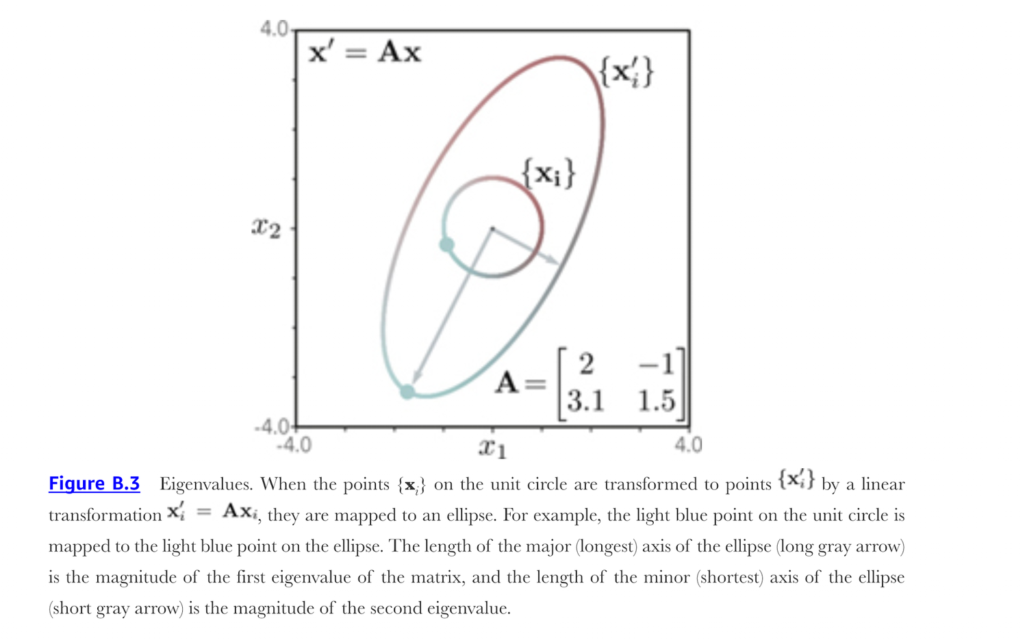
The spectral norm of a square matrix is its largest absolute eigenvalue: the largest change in magnitude the matrix can apply to a unit-length vector, and hence the Lipschitz constant of the transformation. The set of eigenvalues is the eigenspectrum, and it tells us about the magnitude of the scaling applied across all directions. Two scalars summarize that information:
- The determinant \(\lvert \mathbf{A} \rvert\) is the product of the eigenvalues, so it is related to the average scaling the matrix applies. Matrices with small absolute determinants shrink vectors; matrices with large ones grow them. A singular matrix has determinant zero, and there is then at least one direction that gets mapped to the origin — exactly the nullspace of §B.3.6.
- The trace is the sum of the diagonal entries, and also the sum of the eigenvalues.
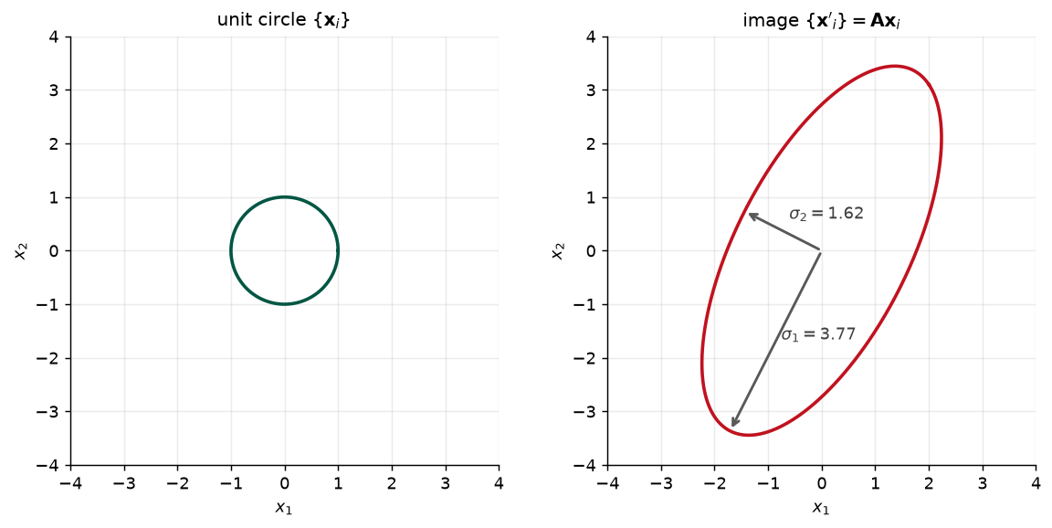
longest / shortest radius measured on the ellipse : 3.7747 / 1.6160
singular values of A                              : 3.7747 / 1.6160
eigenvalues of A                                  : 1.7500+1.7428j, 1.7500-1.7428j
|det A| = 6.1000   product of singular values = 6.1000   product of |eigenvalues| = 6.1000
trace A = 3.5000   sum of eigenvalues = 3.5000
Axis lengths are singular values
The figure’s caption describes the axis lengths as the eigenvalue magnitudes. For this particular \(\mathbf{A}\) the eigenvalues are complex — the matrix rotates as well as stretches — and the printed output shows the semi-axes matching the singular values \(3.77\) and \(1.62\) instead, while both eigenvalues have modulus \(2.47\). The two coincide when \(\mathbf{A}\) is symmetric, which is the case that matters most for us: the loss surfaces of Section 8.5 are governed by a symmetric matrix, and there eigenvalues and singular values are the same numbers. The determinant identity holds either way, and is a good check to keep in your pocket.
4 Special Types of Matrix
Prince §B.4.
Inverting a general \(\mathbf{A} \in \mathbb{R}^{D \times D}\) costs \(\mathcal{O}[D^3]\), as does computing its determinant. Matrices with structure are much cheaper, and a surprising amount of practical numerical work consists of arranging for the matrices you have to be one of these.
| Type | Structure | What it buys |
|---|---|---|
| Diagonal | zeros off the principal diagonal | inverse is \(1/d_{ii}\) entrywise; \(\lvert\mathbf{A}\rvert = \prod_i d_{ii}\) |
| Identity | diagonal of ones | its own inverse; determinant one |
| Triangular | zeros above (lower) or below (upper) the diagonal | invertible in \(\mathcal{O}[D^2]\); determinant is the product of the diagonal |
| Orthogonal | rotation and reflection about the origin | \(\mathbf{A}^{-1} = \mathbf{A}^{T}\); all \(\lvert\lambda_i\rvert = 1\); \(\lvert\mathbf{A}\rvert = \pm 1\) |
| Permutation | one entry equal to one in each row and column | orthogonal, so \(\mathbf{A}^{-1} = \mathbf{A}^{T}\); \(\lvert\mathbf{A}\rvert = \pm 1\) |
An orthogonal matrix maps the circle of fig. 2 to another circle of the same radius, rotated and possibly reflected — which is exactly why all its eigenvalues have magnitude one. A permutation matrix is a special case: it permutes the entries of a vector, as in Prince’s example (B.16),
\[ \begin{bmatrix} 0 & 1 & 0 \\ 0 & 0 & 1 \\ 1 & 0 & 0 \end{bmatrix} \begin{bmatrix} a \\ b \\ c \end{bmatrix} = \begin{bmatrix} b \\ c \\ a \end{bmatrix}. \tag{8}\]
Each shortcut in the table, checked in turn:
diagonal : inverse is the reciprocal : True | det == product of diagonal : True
triangular: det == product of diagonal : True
orthogonal: A^-1 == A^T : True | |eigenvalues| : [1. 1. 1. 1. 1.] | det : 1.0

permutation (B.16): [2. 3. 1.] -> ['b' 'c' 'a']
permutation: P^-1 == P^T : True
5 Linear Equations in Matrix Form
Prince §B.4.5–§B.4.6.
Linear algebra is the mathematics of linear functions, which have the form
\[ f[z_1, z_2, \dots z_D] = \phi_1 z_1 + \phi_2 z_2 + \dots \phi_D z_D, \tag{9}\]
where \(\phi_1, \dots, \phi_D\) are the parameters that define the function. We almost always add a constant \(\phi_0\) to the right-hand side. Strictly that makes the function affine rather than linear, but machine learning calls it linear anyway, and so will we.
Now take a collection of such functions,
\[ \begin{aligned} y_1 &= \phi_{10} + \phi_{11} z_1 + \phi_{12} z_2 + \phi_{13} z_3 \\ y_2 &= \phi_{20} + \phi_{21} z_1 + \phi_{22} z_2 + \phi_{23} z_3 \\ y_3 &= \phi_{30} + \phi_{31} z_1 + \phi_{32} z_2 + \phi_{33} z_3, \end{aligned} \tag{10}\]
and stack them:
\[ \begin{bmatrix} y_1 \\ y_2 \\ y_3 \end{bmatrix} = \begin{bmatrix} \phi_{10} \\ \phi_{20} \\ \phi_{30} \end{bmatrix} + \begin{bmatrix} \phi_{11} & \phi_{12} & \phi_{13} \\ \phi_{21} & \phi_{22} & \phi_{23} \\ \phi_{31} & \phi_{32} & \phi_{33} \end{bmatrix} \begin{bmatrix} z_1 \\ z_2 \\ z_3 \end{bmatrix}, \tag{11}\]
or, for short,
\[ \mathbf{y} = \boldsymbol{\phi}_0 + \boldsymbol{\Phi}\mathbf{z}, \qquad y_i = \phi_{i0} + \sum_{j=1}^{3} \phi_{ij} z_j. \tag{12}\]
The printed equation (B.18) opens its third row with \(\phi_{20}\) where the matrix form (B.19) has \(\phi_{30}\). eq. 10 above is written with \(\phi_{30}\), which is what the rest of the appendix — and the notebook — assume.
eq. 12 is the single most important object in this course. Every fully connected layer of every network from Chapter 3 onward computes exactly this and then applies a nonlinearity to the result. torch.nn.Linear is eq. 12: its weight attribute is \(\boldsymbol{\Phi}\) and its bias is \(\boldsymbol{\phi}_0\).
scalar form : [-3.    3.    3.75]
matrix form : [-3.    3.    3.75]
identical   : True
nn.Linear   : [-3.    3.    3.75]
A layer applied to a whole batch of inputs is the same equation with \(\mathbf{z}\) replaced by a matrix whose columns are the examples — which is why training on a batch of 256 costs barely more than training on one:
input batch : (3, 256)  output batch: (3, 256)
column 7 matches the single-input computation: True
6 Matrix Calculus
Prince §B.5.
If \(y = f[x]\) is a scalar function of a scalar, the derivative \(\partial y / \partial x\) says how \(y\) changes for a small change in \(x\). The same idea extends upward, and the only thing to keep straight is the shape of the answer:
| Function | Argument | Derivative \(\partial y / \partial \mathbf{x}\) |
|---|---|---|
| \(y = \mathrm{f}[\mathbf{x}]\), \(y \in \mathbb{R}\) | \(\mathbf{x} \in \mathbb{R}^{D}\) | a \(D\)-dimensional vector with \(i^{th}\) element \(\partial y / \partial x_i\) |
| \(\mathbf{y} = \mathbf{f}[\mathbf{x}]\), \(\mathbf{y} \in \mathbb{R}^{D_y}\) | \(\mathbf{x} \in \mathbb{R}^{D_x}\) | a \(D_x \times D_y\) matrix with element \((i, j)\) equal to \(\partial y_j / \partial x_i\) — the Jacobian, sometimes written \(\nabla_{\mathbf{x}}\mathbf{y}\) |
| \(\mathbf{y} = \mathbf{f}[\mathbf{X}]\), \(\mathbf{y} \in \mathbb{R}^{D_y}\) | \(\mathbf{X} \in \mathbb{R}^{D_1 \times D_2}\) | a 3D tensor of the \(\partial y_j / \partial x_{ik}\) |
These have superficially similar forms to the scalar case:
\[ y = ax \quad \longrightarrow \quad \frac{\partial y}{\partial x} = a, \tag{13}\]
and
\[ \mathbf{y} = \mathbf{A}\mathbf{x} \quad \longrightarrow \quad \frac{\partial \mathbf{y}}{\partial \mathbf{x}} = \mathbf{A}^{T}. \tag{14}\]
Why the transpose in eq. 14
Prince’s table puts \(\partial y_j / \partial x_i\) at position \((i, j)\): inputs index the rows, outputs the columns. That is denominator layout, and it is what makes the answer \(\mathbf{A}^T\) rather than \(\mathbf{A}\). PyTorch, JAX, and most autodiff libraries use the opposite (numerator) layout, so jacobian returns \(\mathbf{A}\). Neither is wrong; they are transposes of each other. When a gradient in your code has the wrong shape, layout is the first thing to suspect.
The Jacobian of \(\mathbf{y} = \mathbf{A}\mathbf{x}\), and the derivative of a scalar function of a vector:
torch jacobian shape (numerator layout, D_y x D_x): (2, 3)
equals A            : True
its transpose is Prince's dy/dx = A^T, shape (3, 2)

d/dx of ||x||^2 : [ 2. -4.  6.]  expected 2x : [ 2. -4.  6.]
Automatic differentiation is what makes deep learning practical: we write the forward computation, and the library assembles the derivative by applying the chain rule to the operations we used. Chapter 7 opens up the machinery. For now it is enough to trust it — and to verify it, which is what the two lines below do, on the object we actually care about: the gradient of a loss.
autograd : [20.312  -5.7116 -8.9976]
analytic : [20.312  -5.7116 -8.9976]
agree    : True
7 Supervised Learning, Revisited
Prince §2.1, pp. 17–18.
With the notation settled, Chapter 2 reads differently the second time. A supervised model is a function that takes an input and returns a prediction,
\[ \mathbf{y} = \mathbf{f}[\mathbf{x}], \tag{15}\]
and running it to get \(\mathbf{y}\) from \(\mathbf{x}\) is called inference. The model is just a mathematical equation of fixed form, so it describes a whole family of possible relationships between inputs and outputs; the parameters \(\boldsymbol{\phi}\) specify which member of that family we have:
\[ \mathbf{y} = \mathbf{f}[\mathbf{x}, \boldsymbol{\phi}]. \tag{16}\]
To train or learn a model is to find parameters that describe the true relationship. A learning algorithm takes a training set of \(I\) input/output pairs \(\{\mathbf{x}_i, \mathbf{y}_i\}\) and manipulates \(\boldsymbol{\phi}\) until the inputs predict their corresponding outputs as closely as possible. We measure “as closely as possible” with a scalar loss \(L[\boldsymbol{\phi}]\) and minimize it:
\[ \hat{\boldsymbol{\phi}} = \operatorname*{argmin}_{\boldsymbol{\phi}} \big[ L[\boldsymbol{\phi}] \big]. \tag{17}\]
If the loss is small after this minimization, we have found parameters that predict the training outputs accurately. That is not the same as a useful model, so we then run it on separate test data to see how well it generalizes to examples it did not observe during training. If that performance is adequate, we are ready to deploy.
Three verbs, in order, for the rest of the semester: train, then test, then infer.
8 Linear Regression, in Matrix Form
Prince §2.2, pp. 18–22.
8.1 The model
Prince §2.2.1, p. 18; figure on p. 19.
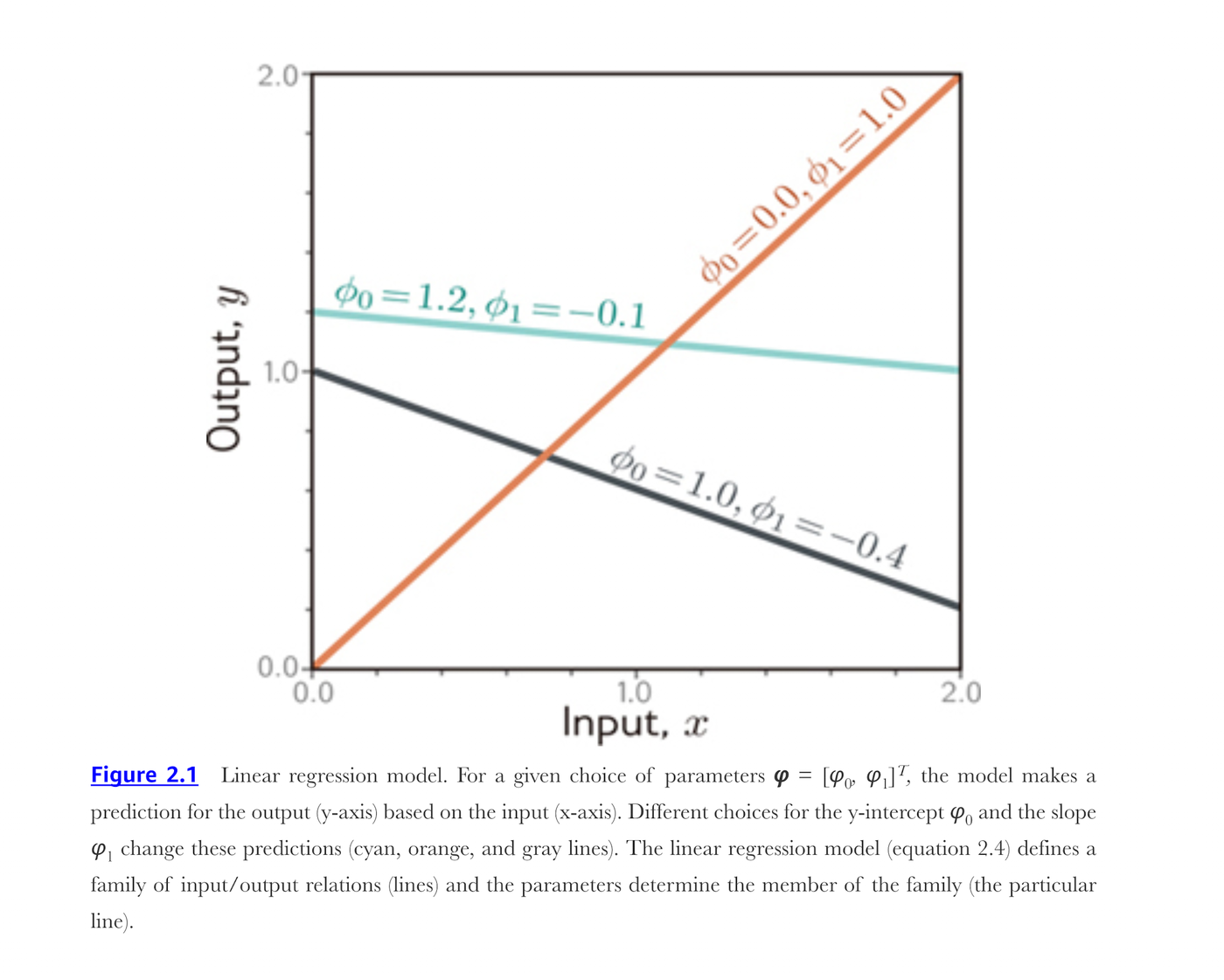
A 1D linear regression model describes the relationship between input \(x\) and output \(y\) as a straight line:
\[ y = f[x, \boldsymbol{\phi}] = \phi_0 + \phi_1 x. \tag{18}\]
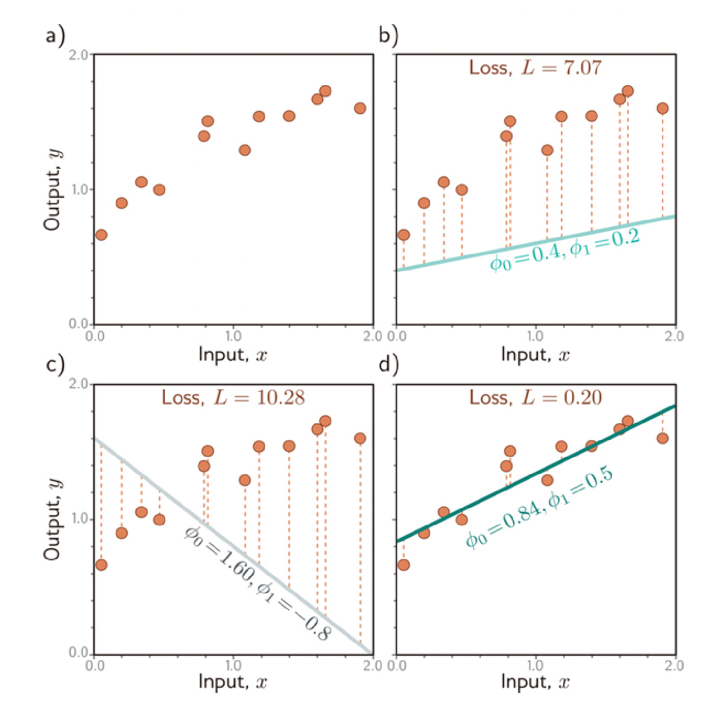
This is eq. 9 with \(D = 1\), and it has two parameters: \(\boldsymbol{\phi} = [\phi_0, \phi_1]^T\), a \(y\)-intercept and a slope. fig. 4 shows the family: eq. 18 defines all possible lines, and the parameters pick one.
8.2 The loss
Prince §2.2.2, pp. 19–21; figures on pp. 20–21.
The loss quantifies the mismatch between predictions and observations. Sum the squared deviations over the \(I\) training pairs:
\[ L[\boldsymbol{\phi}] = \sum_{i=1}^{I} \big( f[x_i, \boldsymbol{\phi}] - y_i \big)^2 = \sum_{i=1}^{I} \big( \phi_0 + \phi_1 x_i - y_i \big)^2. \tag{19}\]
fig. 5 shows three candidate lines against the same twelve points, with the deviations drawn as dashed verticals and the resulting loss printed above each panel. The visual quality of the fit and the value of the loss agree, which is the whole point: the loss is a number that stands in for “looks right”.
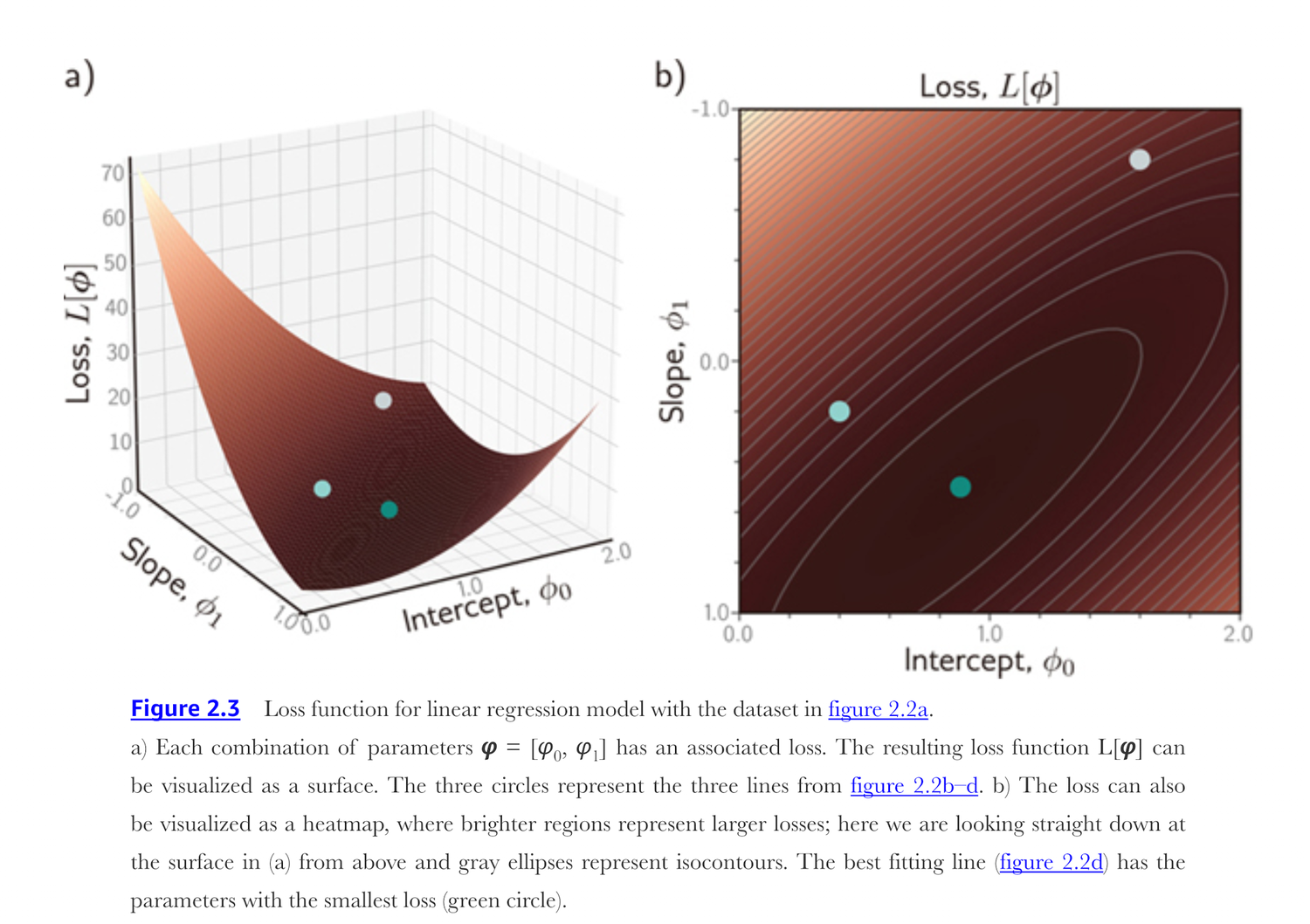
Because the model has only two parameters, the loss can be drawn in full, as a surface over \((\phi_0, \phi_1)\) or as a heatmap seen from above. fig. 6 does both. Every point in those pictures is one line in fig. 5, and the bottom of the bowl is the best line.
Training is eq. 17 applied to eq. 19:
\[ \hat{\boldsymbol{\phi}} = \operatorname*{argmin}_{\boldsymbol{\phi}} \left[ \sum_{i=1}^{I} \big( \phi_0 + \phi_1 x_i - y_i \big)^2 \right]. \tag{20}\]
8.3 The same loss, in matrix form
Now use Appendix B. Stack the \(I\) inputs into a design matrix \(\mathbf{X} \in \mathbb{R}^{I \times 2}\) whose first column is all ones and whose second column holds the inputs. Then all \(I\) predictions are one matrix–vector product, \(\mathbf{X}\boldsymbol{\phi}\), and eq. 19 becomes a squared Euclidean norm:
\[ L[\boldsymbol{\phi}] = \lVert \mathbf{X}\boldsymbol{\phi} - \mathbf{y} \rVert^2 . \tag{21}\]
Differentiating with the rules of §B.5 and setting the result to zero gives the normal equations \(\mathbf{X}^T\mathbf{X}\hat{\boldsymbol{\phi}} = \mathbf{X}^T\mathbf{y}\), which is Prince’s problem 2.2 done in two lines instead of a page of algebra. The gradient we will need in a moment is
\[ \frac{\partial L}{\partial \boldsymbol{\phi}} = 2\mathbf{X}^T(\mathbf{X}\boldsymbol{\phi} - \mathbf{y}). \tag{22}\]
Here is a small process dataset to fit: the cure temperature of a composite panel against the tensile strength of the finished part.
design matrix: (24, 2)  first two rows:
 [[  1.         164.52268379]
 [  1.         164.20898069]]

normal equations X^T X phi = X^T y:
X^T X =
 [[2.4000000e+01 4.1026700e+03]
 [4.1026700e+03 7.0988862e+05]]
8.4 Training, three ways
Prince §2.2.3, p. 22; figure on p. 23.
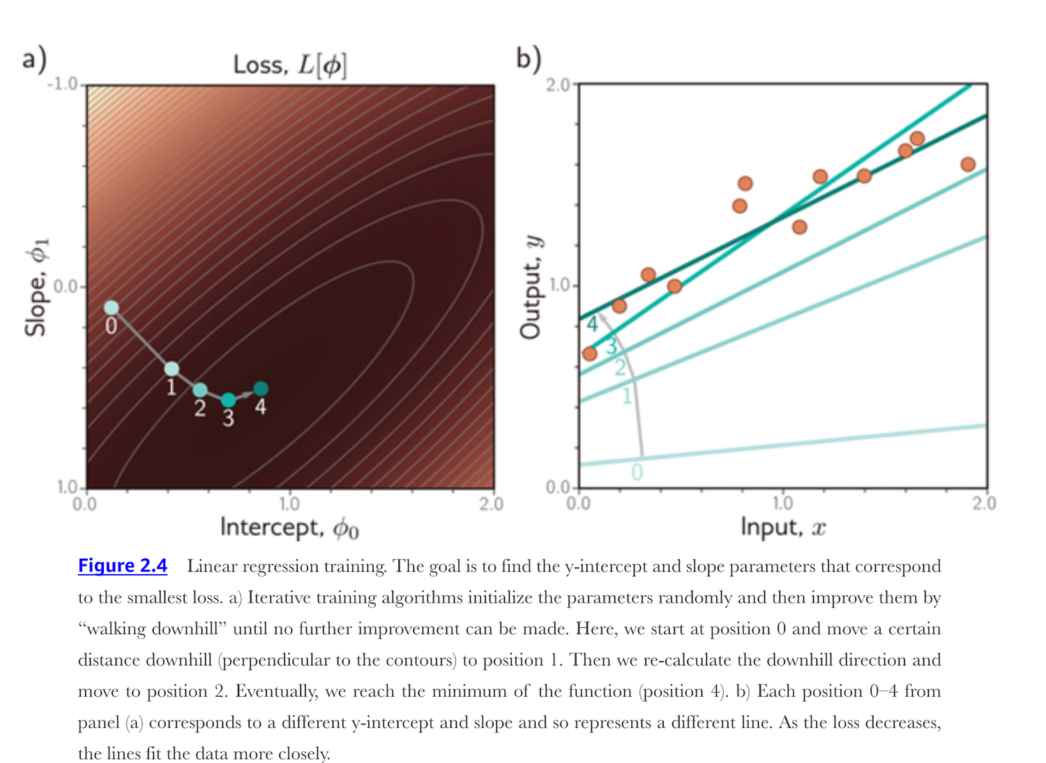
The process of finding the parameters that minimize the loss is called model fitting, training, or learning. The basic method is to choose the initial parameters randomly and then improve them by “walking downhill” on the loss function until we reach the bottom: measure the gradient of the surface at the current position, take a step in the most steeply downhill direction, and repeat until the gradient is flat and we can improve no further. fig. 7 shows five such steps, and the five lines they correspond to.
Linear regression does not actually need the iterative approach — it has a closed-form solution — but every model after Chapter 3 does, so it is worth running all three and comparing what comes back.
method                     phi_0     phi_1        loss
closed form              19.1998    0.3825    122.7487
gradient descent          0.2238    0.4921    226.9542
PyTorch (Adam)           19.1961    0.3834    123.3793
The closed form and PyTorch land on the same line. Plain gradient descent, given a learning rate that looks perfectly reasonable, does not: after twenty thousand steps its slope is still nearly 30% too large, its intercept is nowhere near the right value, and its loss is close to double the minimum. That failure is not a bug and it is not cured by being patient. It is the most useful thing on this page, so the next section takes it apart.
8.5 Why the iterative methods struggle
The loss eq. 21 is a quadratic bowl, and the matrix that describes its curvature is \(\partial^2 L / \partial \boldsymbol{\phi}^2 = 2\mathbf{X}^T \mathbf{X}\) — symmetric, so §B.3.7’s eigenvalues and singular values coincide here. Its eigenspectrum is the shape of the bowl: the largest eigenvalue is the curvature in the steepest direction, the smallest is the curvature along the floor of the valley, and their ratio is the condition number. Gradient descent is stable only for step sizes below \(2/\lambda_{\max}\), and it makes progress along the valley floor at a rate set by \(\lambda_{\min}\). A large ratio therefore means a step size chosen small enough to be safe is far too small to make progress.
Cure temperature runs from 140 to 200, so the second column of \(\mathbf{X}\) is enormous compared to the column of ones, and the bowl is a knife-edge ravine. Standardizing the input — subtracting the mean and dividing by the standard deviation — makes the two columns orthogonal and equal in length, which turns the ravine into a perfectly round bowl.
raw            Hessian eigenvalues       0.5788   1419824.6693   condition number    2453231.2
standardized   Hessian eigenvalues      48.0000        48.0000   condition number          1.0

largest stable step size -- raw: 1.268e-06, standardized: 3.750e-02
steps to get within 1% of the optimum -- raw: None, standardized: 27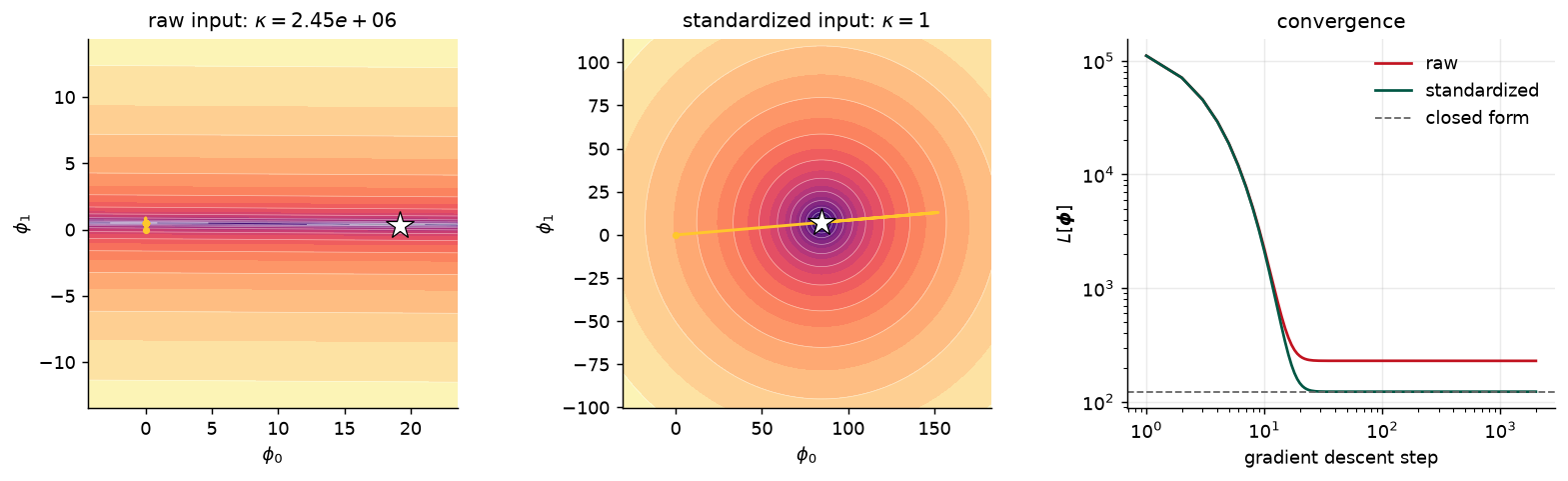
Every trick in Chapter 7 — initialization schemes, normalization layers, momentum, Adam — exists to fight the effect this cell demonstrates on two parameters. Standardizing your inputs is the cheapest version of that fight, and it costs two lines.
8.6 Testing
Prince §2.2.4, p. 22.
Having trained the model, we want to know how it will perform in the real world, so we compute the loss on a separate set of test data. How well accuracy generalizes depends partly on how representative and complete the training data is, and partly on how expressive the model is. A model as simple as a line may be unable to capture the true relationship, which is underfitting. A very expressive model may instead describe statistical peculiarities of the training data that are atypical, leading to unusual predictions, which is overfitting.
To see both, fit polynomials of three different degrees to our twenty-four panels and then score each one on a fresh batch of two hundred parts from the same process. Degree 1 is eq. 18; degree 0 is a horizontal line, which cannot represent a trend at all; degree 12 has enough freedom to weave through most of the training points.
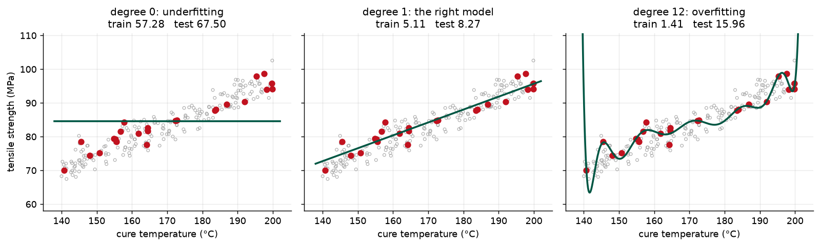
The ordering of those six numbers is the whole of Chapter 8 in miniature. Training loss falls monotonically as the model gets more expressive, so it cannot be used to choose a model. Test loss falls and then rises, and the model we want is at the bottom of that curve. Notice where the degree-12 model does its damage: the curve swings hardest near the ends of the temperature range, where a high-degree polynomial has the fewest points holding it down. Chapter 9 answers this with regularization; for now the practical rule is that a model must be scored on data it has never seen. We were able to make more parts here; when you cannot, you hold part of the dataset back instead, which is what Chapter 8 is about.
9 Summary
Prince §2.3, p. 22, and Appendix B.
Appendix B gives us four things we will use every week. Vectors, matrices, and tensors are arrays distinguished only by how many indices they carry. Norms measure size, dot products measure alignment, and the eigenspectrum, determinant, and trace summarize what a linear map does to space. Structured matrices — diagonal, triangular, orthogonal, permutation — replace \(\mathcal{O}[D^3]\) work with something cheaper. And a system of linear equations collapses to \(\mathbf{y} = \boldsymbol{\phi}_0 + \boldsymbol{\Phi}\mathbf{z}\), which is exactly what one layer of a neural network computes.
Matrix calculus tells us the shape of a derivative before we compute it, and autodiff computes it for us; the only trap is layout, where Prince’s \(\partial\mathbf{y}/\partial\mathbf{x} = \mathbf{A}^T\) and PyTorch’s Jacobian \(\mathbf{A}\) are transposes of one another.
A supervised model is a function \(\mathbf{y} = \mathbf{f}[\mathbf{x}, \boldsymbol{\phi}]\) relating inputs to outputs, with \(\boldsymbol{\phi}\) selecting one member of a family. To train it, we define a loss \(L[\boldsymbol{\phi}]\) over a training set \(\{\mathbf{x}_i, \mathbf{y}_i\}\) quantifying the mismatch between the model’s predictions and the observed outputs, then search for the parameters that minimize it. We evaluate on separate test data to see how it generalizes.
Linear regression has the obvious drawback that it can only describe the relationship between input and output as a straight line. Chapters 3–9 expand on these ideas: shallow neural networks are only slightly more complex than linear regression but describe a much larger family of input/output relationships, and deep networks are just as expressive but describe complex functions with fewer parameters and work better in practice. Chapter 5 investigates loss functions for different tasks and reveals the theoretical underpinnings of the least-squares loss; Chapters 6 and 7 discuss the training process; Chapter 8 discusses how to measure model performance; and Chapter 9 considers regularization techniques, which aim to improve that performance.
Discriminative and generative models
The models \(\mathbf{y} = \mathbf{f}[\mathbf{x}, \boldsymbol{\phi}]\) in Chapter 2 are discriminative: they predict an output from real-world measurements. The alternative is a generative model \(\mathbf{x} = \mathbf{g}[\mathbf{y}, \boldsymbol{\phi}]\), which computes the measurements as a function of the output and lets us build in prior knowledge about how the data were created. Inference then requires inverting the equation, which may be hard. Prince’s verdict, on p. 23: the advantage gained from exploiting prior knowledge in generative models “is usually trumped by learning very flexible discriminative models with large amounts of training data.” Problem 2.3 below asks you to try it both ways.
Next: Chapter 3 replaces the straight line of eq. 18 with a shallow neural network — eq. 12, followed by a ReLU, followed by eq. 12 again.
10 Exercises
1. A quality inspection station records 8 sensor readings for each of 500 parts. Write down the shape of the design matrix, of a parameter matrix \(\boldsymbol{\Phi}\) for a layer producing 3 outputs per part, of the bias \(\boldsymbol{\phi}_0\), and of the output. Then state which of eq. 1, eq. 4, and eq. 12 you used to check each one.
2. Show that \((\mathbf{A}\mathbf{B}\mathbf{C})^T = \mathbf{C}^T\mathbf{B}^T \mathbf{A}^T\) using eq. 1 twice. Then explain, in one sentence about shapes, why no other ordering could be correct.
3. Two vibration spectra \(\mathbf{a}\) and \(\mathbf{b}\) have \(\lVert\mathbf{a}\rVert = 3\), \(\lVert\mathbf{b}\rVert = 5\), and \(\mathbf{a}^T \mathbf{b} = 7.5\). What is the angle between them? If a third spectrum \(\mathbf{c} = 4\mathbf{a}\), what are \(\mathbf{a}^T\mathbf{c}\) and the angle between \(\mathbf{a}\) and \(\mathbf{c}\)? Which of these two numbers would you use to compare spectra of different intensities, and why?
4. A matrix \(\mathbf{A} \in \mathbb{R}^{3 \times 5}\) maps a 5-dimensional input to a 3-dimensional output. What is the largest possible dimension of its column space, and the smallest possible dimension of its nullspace? Give a concrete consequence for a sensor-fusion model that compresses 5 measurements to 3 features.
5. A \(2 \times 2\) matrix has \(\det[\mathbf{A}] = 0.01\) and trace 2.1. Find its eigenvalues. Is the transformation better described as a shrink, a stretch, or a shear? What happens to the unit circle under it?
6. Computational. In the notebook, modify the unit_ball function behind fig. 1 to plot \(p = 0.5\) alongside \(p = 1\) and \(p = 2\). The result is not convex. Read §B.3.2 again and explain which property in eq. 2 fails, and why that matters if you wanted to use \(\lVert\cdot\rVert_{0.5}\) as a regularizer.
7. Computational. Take the conditioning experiment in fig. 8 and change the units of the input from degrees Celsius to kelvin (add 273.15). Report the condition number and the number of steps to converge before and after. Then explain why the closed-form solution is unaffected while gradient descent is crippled.
8. (UDL 2.1) To walk “downhill” on the loss function eq. 19, we measure its gradient with respect to the parameters \(\phi_0\) and \(\phi_1\). Calculate expressions for the slopes \(\partial L / \partial \phi_0\) and \(\partial L / \partial \phi_1\). Check them against eq. 22 by evaluating both on the cure-temperature data.
9. (UDL 2.2) Show that the minimum of the loss function can be found in closed form by setting the expressions for the derivatives from problem 8 to zero and solving for \(\phi_0\) and \(\phi_1\). Confirm that your answer is the normal equations of eq. 21. Note that this works for linear regression but not for more complex models; this is why we use iterative model fitting methods like gradient descent.
10. (UDL 2.3*) Consider reformulating linear regression as a generative model, so we have \(x = g[y, \boldsymbol{\phi}] = \phi_0 + \phi_1 y\). What is the new loss function? Find an expression for the inverse function \(y = g^{-1}[x, \boldsymbol{\phi}]\) that we would use to perform inference. Will this model make the same predictions as the discriminative version for a given training dataset \(\{x_i, y_i\}\)? One way to establish this is to write code that fits a line to three data points using both methods and see if the result is the same.
11 Textbook Reference Map
Every part of this page, mapped to Prince, Understanding Deep Learning (MIT Press, 2024) (Prince 2024). Chapter page numbers are those of the printed book; Appendix B is cited by section.
| This page | Prince section | Pages | Figures used |
|---|---|---|---|
| Vectors, Matrices, and Tensors | §B.3 | App. B | — |
| — Transpose | §B.3.1 | App. B | — |
| — Vector and matrix norms | §B.3.2 | App. B | — |
| — Products | §B.3.3, §B.3.4 | App. B | — |
| — Inverse | §B.3.5 | App. B | — |
| — Subspaces | §B.3.6 | App. B | — |
| — Eigenspectrum, determinant, and trace | §B.3.7, §B.3.8 | App. B | B.3 |
| Special Types of Matrix | §B.4.1–§B.4.4 | App. B | — |
| Linear Equations in Matrix Form | §B.4.5, §B.4.6 | App. B | — |
| Matrix Calculus | §B.5 | App. B | — |
| Supervised Learning, Revisited | §2.1 | 17–18 | — |
| Linear Regression, in Matrix Form | §2.2 | 18–22 | — |
| — The model | §2.2.1 | 18 | 2.1 (p. 19) |
| — The loss | §2.2.2 | 19–21 | 2.2 (p. 20), 2.3 (p. 21) |
| — Training, three ways | §2.2.3 | 22 | 2.4 (p. 23) |
| — Testing | §2.2.4 | 22 | — |
| Summary | §2.3 and Notes | 22–23 | — |
| Exercises 8–10 | Problems 2.1–2.3 | 24 | — |
Equations on this page correspond to Prince as follows: eq. 1 is his (B.7), eq. 2 is (B.8), eq. 3 is (B.9), eq. 4 is (B.10), eq. 5 is (B.11), eq. 6 is (B.12), eq. 7 is (B.13), eq. 8 is (B.16), eq. 9 is (B.17), eq. 10 is (B.18), eq. 11 and eq. 12 are (B.19), eq. 13 is (B.20), and eq. 14 is (B.21). From Chapter 2, eq. 15 is his (2.1), eq. 16 is (2.2), eq. 17 is (2.3), eq. 18 is (2.4), eq. 19 is (2.5), and eq. 20 is (2.6). eq. 21 and eq. 22 are the matrix forms of (2.5) and of the answer to his problem 2.1; they do not appear in the book.
Figure credits
Figure B.3 and figures 2.1–2.4 are reproduced unaltered from Prince, Understanding Deep Learning (MIT Press, 2024), which is distributed under a Creative Commons CC-BY-NC-ND license, and are used here for non-commercial classroom instruction. All other figures on this page are generated by the code in this week’s notebook.
12 Further Reading
- Prince, Understanding Deep Learning, Appendix B and Chapter 2 (Prince 2024) — the assigned reading.
- ▶ UDL notebook 1.1 — Background mathematics and ▶ UDL notebook 2.1 — Supervised learning — Prince’s own Colab notebooks for this material.
- ▶ This week’s notebook — every cell above, in one Colab file.
- Deisenroth, Faisal & Ong, Mathematics for Machine Learning (2020) — the book to open if Appendix B moves too fast. Chapters 2–5 cover everything on this page at length, and it is free online.
- Strang, Introduction to Linear Algebra — the standard reference for subspaces, the four fundamental subspaces, and eigendecomposition.
- Petersen & Pedersen, The Matrix Cookbook — a lookup table of matrix derivatives; the companion to §B.5 when you need an identity in a hurry.
- Trefethen & Bau, Numerical Linear Algebra — why we solve rather than invert, and what a condition number really costs.
- The PyTorch tensor tutorial and autograd tutorial — the official versions of the code in this note.
References
Prince, Simon J. D. 2024. Understanding Deep Learning. MIT Press. https://udlbook.github.io/udlbook/.