 iterate       0       1       2       3       4       5       6       7       8
    loss   6.121   2.872   1.386   0.707   0.396   0.254   0.189   0.160   0.146

closed-form optimum (normal equations): loss 0.1346Week 6 · Sessions 11–12 · September 29 & October 1, 2026
Every section below opens with the section number and page range it covers in Prince, Understanding Deep Learning (MIT Press, 2024). Page numbers are those of the printed book. Figures taken from the textbook are captioned with their original figure number and page; figures generated by the code behind this page are ours. A complete cross-reference table appears in Section 12.
By the end of this week you should be able to:
torch.optim.SGD and torch.optim.Adam, and translate between Prince’s momentum convention and PyTorch’s.This page shows the figures and results; the Python behind them is not printed here. All of it — every cell, in the order the note uses it — is in a notebook you can open in the browser with nothing to install:
Colab gives you a Python environment with NumPy, matplotlib, and PyTorch already installed. In Colab, run a cell with Shift+Enter. If you prefer to work locally, pip install -r requirements.txt from the course repository gives you the same environment.
Prince, Chapter 6 opening, p. 77.
Three chapters have now built the pieces. Weeks 3 and 4 gave families of piecewise linear functions, one member per setting of the parameters \(\boldsymbol{\phi}\). Week 5 gave the loss \(L[\boldsymbol{\phi}]\), a single number measuring how badly a given member describes the training data. What is missing is the search: finding the parameter values that make the loss as small as possible. That search is what we mean by learning the parameters, or equivalently training or fitting the model.
Every method in this course runs the same loop. Choose initial values for the parameters, then repeat two steps:
After enough repetitions we hope to be at the overall minimum. That word is doing real work, and half of this chapter is about why the hope can fail.
This chapter is entirely about step 2: given a gradient, how should we move? Step 1, which for a network with millions of parameters is a substantial computation in its own right, is the backpropagation algorithm of Chapter 7, which also takes up the question this loop quietly begs — where the initial values come from.
Prince §6.1, pp. 77–78.
We have a training set \(\{\mathbf{x}_i, \mathbf{y}_i\}_{i=1}^{I}\), a model \(\mathbf{f}[\mathbf{x}_i, \boldsymbol{\phi}]\), and a loss. The goal of an optimization algorithm is the minimizer
\[ \hat{\boldsymbol{\phi}} = \operatorname*{argmin}_{\boldsymbol{\phi}} \Big[ L[\boldsymbol{\phi}] \Big]. \tag{1}\]
There are many families of optimization algorithms, but the ones used to train neural networks are all iterative: initialize the parameters heuristically, then adjust them repeatedly so that the loss decreases. The simplest member of the family is gradient descent. Starting from parameters \(\boldsymbol{\phi} = [\phi_0, \phi_1, \ldots, \phi_N]^T\), it iterates two steps.
Step 1. Compute the derivatives of the loss with respect to the parameters:
\[ \frac{\partial L}{\partial \boldsymbol{\phi}} = \begin{bmatrix} \dfrac{\partial L}{\partial \phi_0} & \dfrac{\partial L}{\partial \phi_1} & \cdots & \dfrac{\partial L}{\partial \phi_N} \end{bmatrix}^T. \tag{2}\]
Step 2. Update the parameters according to the rule
\[ \boldsymbol{\phi} \longleftarrow \boldsymbol{\phi} - \alpha \cdot \frac{\partial L}{\partial \boldsymbol{\phi}}, \tag{3}\]
where the positive scalar \(\alpha\) sets the size of the change.
The gradient points in the direction in which the loss increases fastest — the uphill direction at the current position. Step 2 therefore moves a small distance downhill, which is the whole reason for the minus sign.
At a minimum the surface must be flat; if it were not, we could keep going downhill. So the gradient there is zero and the updates stop changing anything. In practice we monitor the size of the gradient and stop when it falls below a threshold. Hold on to that stopping rule. It is entirely reasonable, and Section 4.2 will show it can be fooled.
Prince §6.1, p. 78; chapter notes, pp. 92–93; figure on p. 93.
There are two ways to choose \(\alpha\). We can fix it in advance, in which case it is called the learning rate. Or we can perform a line search: having computed the downhill direction, try several values of \(\alpha\) along it and take the one that decreases the loss the most.
The chapter notes explain why the second option exists. With a fixed \(\alpha\), the distance moved is proportional to the size of the gradient, so the method takes long strides where the loss changes fast — exactly where caution is called for — and timid ones where it changes slowly, where it should explore. A line search removes that coupling. One standard procedure is bracketing (fig. 1): keep two interior points inside a search interval, compare the loss at them, discard the end of the interval that cannot contain the minimum, and repeat until the minimum is pinned down.
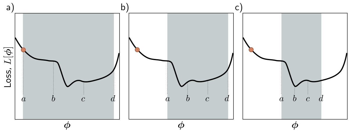
Line search is cheap when one loss evaluation is cheap. For a network trained on millions of examples, every trial value of \(\alpha\) costs a full pass over the data, which is why deep learning almost always uses a fixed learning rate — or a fixed schedule of them — instead.
Prince §6.1.1, pp. 78–80; figure on p. 79.
Start with the model we know best, the 1D linear regression of Chapter 2:
\[ y = \mathrm{f}[x, \boldsymbol{\phi}] = \phi_0 + \phi_1 x, \tag{4}\]
with intercept \(\phi_0\) and slope \(\phi_1\), and the least squares loss over \(I\) pairs,
\[ L[\boldsymbol{\phi}] = \sum_{i=1}^{I} \ell_i = \sum_{i=1}^{I} \big(\mathrm{f}[x_i, \boldsymbol{\phi}] - y_i\big)^2 = \sum_{i=1}^{I} \big(\phi_0 + \phi_1 x_i - y_i\big)^2, \tag{5}\]
where \(\ell_i\) is the contribution of the \(i\)th example. Because the loss is a sum, so is its derivative,
\[ \frac{\partial L}{\partial \boldsymbol{\phi}} = \frac{\partial}{\partial \boldsymbol{\phi}} \sum_{i=1}^{I} \ell_i = \sum_{i=1}^{I} \frac{\partial \ell_i}{\partial \boldsymbol{\phi}}, \tag{6}\]
and each term is
\[ \frac{\partial \ell_i}{\partial \boldsymbol{\phi}} = \begin{bmatrix} \dfrac{\partial \ell_i}{\partial \phi_0} \\[8pt] \dfrac{\partial \ell_i}{\partial \phi_1} \end{bmatrix} = \begin{bmatrix} 2(\phi_0 + \phi_1 x_i - y_i) \\ 2 x_i (\phi_0 + \phi_1 x_i - y_i) \end{bmatrix}. \tag{7}\]
Eq. 6 looks like bookkeeping, but it is the observation the rest of the chapter is built on: the gradient of the whole dataset is a sum of per-example gradients. Stochastic gradient descent will simply stop summing over all of them.
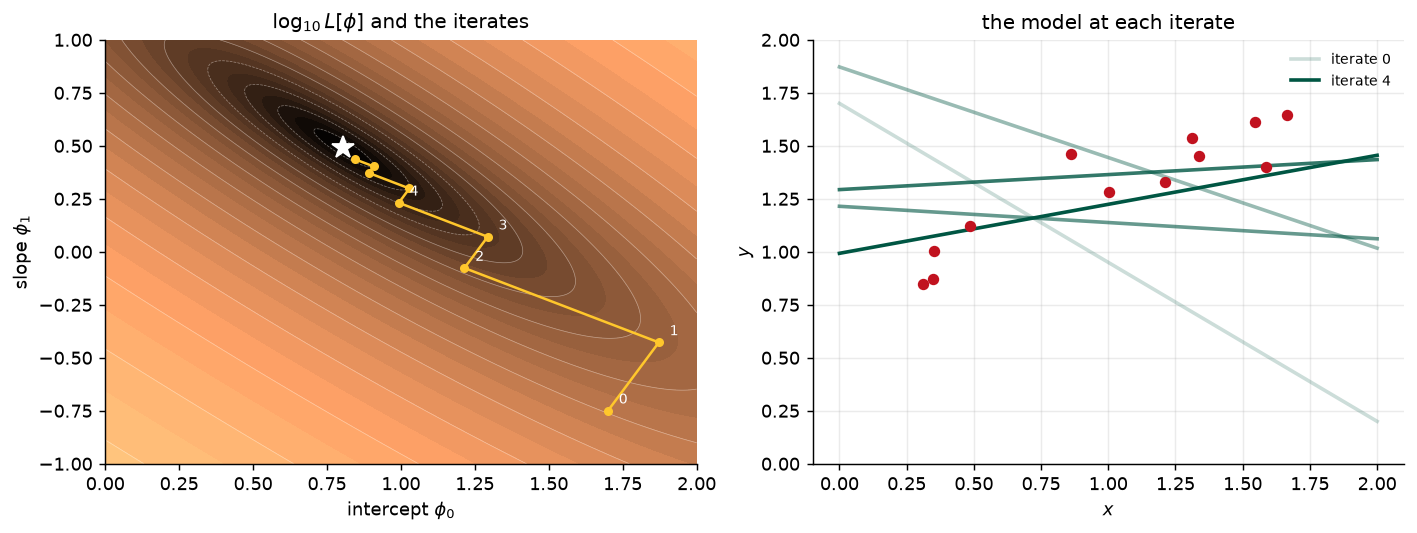
Fig. 2 runs eq. 3 with a line search at every step. Panel (b) shows the loss as a surface, (c) the same surface as a heatmap with the iterates marked, and (d) the line each iterate represents. After four steps the fit is already reasonable.
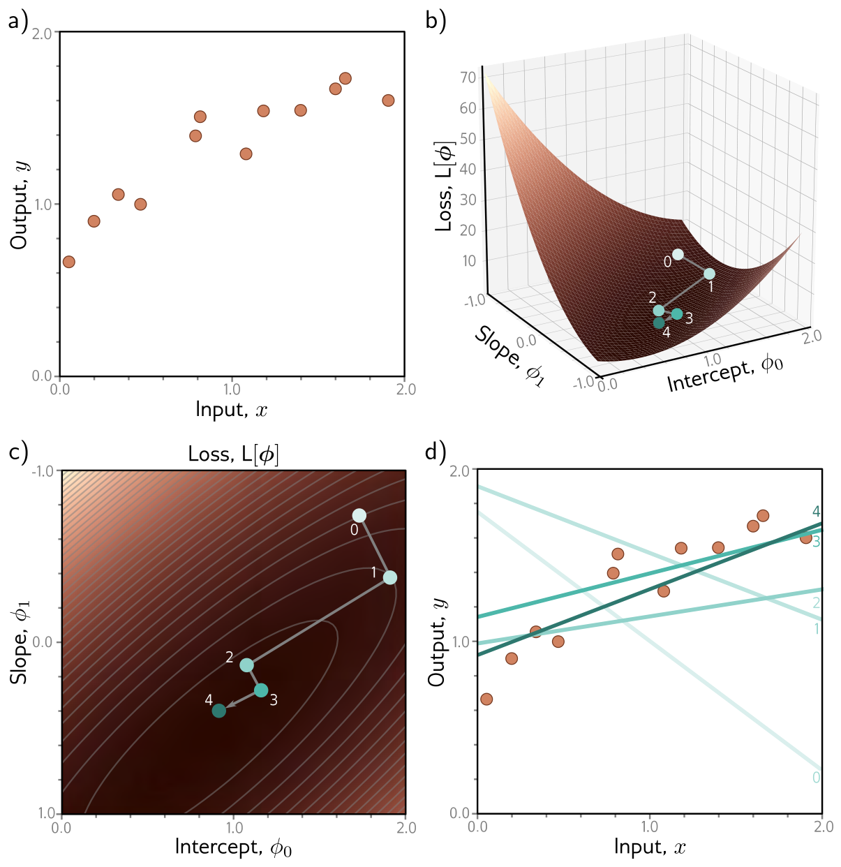
Our version below implements the bracketing search of fig. 1 as a golden-section search and runs it on twelve points of our own.
iterate 0 1 2 3 4 5 6 7 8
loss 6.121 2.872 1.386 0.707 0.396 0.254 0.189 0.160 0.146
closed-form optimum (normal equations): loss 0.1346Two things are worth seeing here. The loss drops by a factor of more than four in the first three steps and then crawls; the last few iterations buy very little. And each step ends exactly where the line search found the bottom of the valley along the current direction, after which the new direction is very different — the path zig-zags even on a perfectly well-behaved bowl. Problem 6.7 asks you why.
The more common choice in deep learning is a fixed learning rate, and here the curvature of the loss sets a hard limit. The Week 2 note showed that for a quadratic loss the Hessian \(2\mathbf{X}^T\mathbf{X}\) describes the shape of the bowl, and that gradient descent is stable only for \(\alpha < 2/\lambda_{\max}\) (Week 2, §“Why the iterative methods struggle”). fig. 4 checks that limit on the same data.
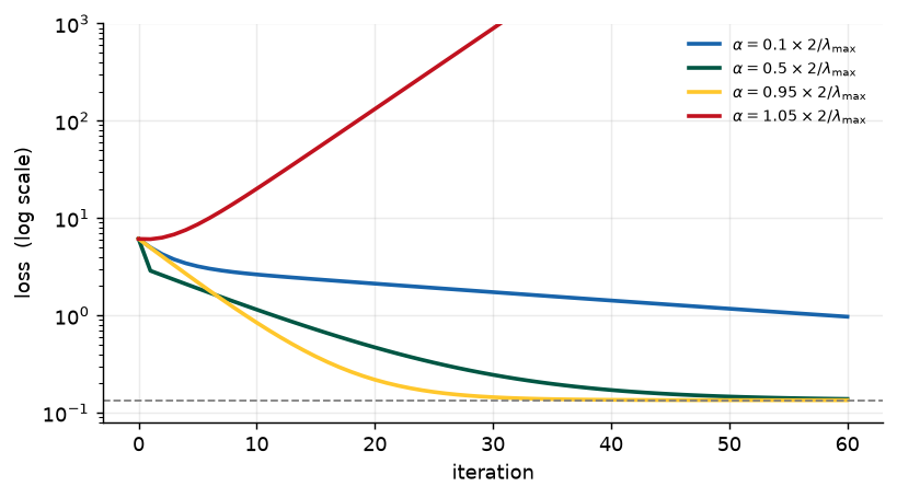
Hessian eigenvalues: [ 2.757 51.216]   condition number 18.6
stability limit 2 / lambda_max = 0.0391
The limit is not a heuristic: on a quadratic, the error along the steepest eigenvector is multiplied by \((1 - \alpha\lambda_{\max})\) at every step, which has magnitude above one exactly when \(\alpha > 2/\lambda_{\max}\). Meanwhile the error along the shallowest direction shrinks by \((1 - \alpha\lambda_{\min})\), so the slowest part of the problem sets the convergence rate while the steepest part sets the step size. Their ratio, the condition number, is the quantity that momentum and Adam will both try to defeat.
Prince §6.1.2, pp. 80–81; figures on p. 81; chapter notes, p. 92.
The linear regression loss has one well-defined global minimum. More precisely it is convex: no chord — no line segment joining two points on the surface — passes below the surface. Convexity has a strong consequence. Wherever we initialize, if we keep walking downhill we are bound to reach the minimum; the training procedure cannot fail.
The chapter notes give the algebraic test. Collect the second derivatives into the Hessian,
\[ \mathbf{H}[\boldsymbol{\phi}] = \begin{bmatrix} \dfrac{\partial^2 L}{\partial \phi_0^2} & \dfrac{\partial^2 L}{\partial \phi_0 \partial \phi_1} & \cdots & \dfrac{\partial^2 L}{\partial \phi_0 \partial \phi_N} \\[8pt] \dfrac{\partial^2 L}{\partial \phi_1 \partial \phi_0} & \dfrac{\partial^2 L}{\partial \phi_1^2} & \cdots & \dfrac{\partial^2 L}{\partial \phi_1 \partial \phi_N} \\ \vdots & \vdots & \ddots & \vdots \\ \dfrac{\partial^2 L}{\partial \phi_N \partial \phi_0} & \dfrac{\partial^2 L}{\partial \phi_N \partial \phi_1} & \cdots & \dfrac{\partial^2 L}{\partial \phi_N^2} \end{bmatrix}. \tag{8}\]
If \(\mathbf{H}\) is positive definite — all eigenvalues positive — for every \(\boldsymbol{\phi}\), the function is convex: a smooth bowl with a single global minimum and no local minima or saddle points. Problem 6.2 asks you to prove this for linear regression.
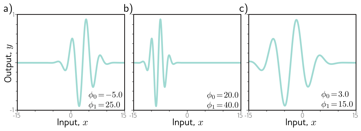
Unfortunately the loss functions of almost all nonlinear models, shallow and deep networks included, are non-convex. A network’s loss is impossible to draw, so Prince studies a nonlinear model with only two parameters, the Gabor model:
\[ \mathrm{f}[x, \boldsymbol{\phi}] = \sin\big[\phi_0 + 0.06 \cdot \phi_1 x\big] \cdot \exp\left[ \frac{-(\phi_0 + 0.06 \cdot \phi_1 x)^2}{32.0} \right]. \tag{9}\]
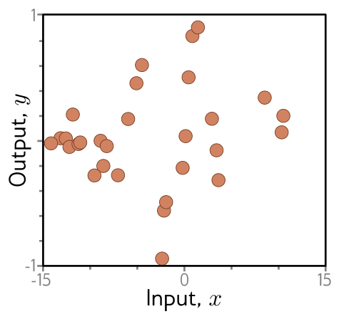
It multiplies an oscillating sinusoid by a decaying exponential, so the oscillation dies away from its center (fig. 5). The parameter \(\phi_0 \in \mathbb{R}\) sets the position of the center and \(\phi_1 \in \mathbb{R}^+\) squeezes or stretches the function along the \(x\)-axis. Fitting it to \(I\) training pairs (fig. 6) by least squares means minimizing
\[ L[\boldsymbol{\phi}] = \sum_{i=1}^{I} \big(\mathrm{f}[x_i, \boldsymbol{\phi}] - y_i\big)^2. \tag{10}\]
The Hessian test does more than certify convexity. At any point where the gradient is zero — a critical point — its eigenvalues classify what kind of point it is: all positive means a minimum, all negative a maximum, and a mixture a saddle point, with the positive eigenvalues marking directions in which we sit at a minimum and the negative ones directions in which we sit at a maximum.
That suggests an experiment the chapter does not run: find every critical point of the Gabor loss and classify each one. Newton’s method — which the chapter notes describe as stepping by \(-\mathbf{H}^{-1}\,\partial L/\partial \boldsymbol{\phi}\) — is the right tool, precisely because of the flaw the notes point out: it heads for the nearest critical point, whatever kind it is. Run from a grid of starting points, it finds them all.
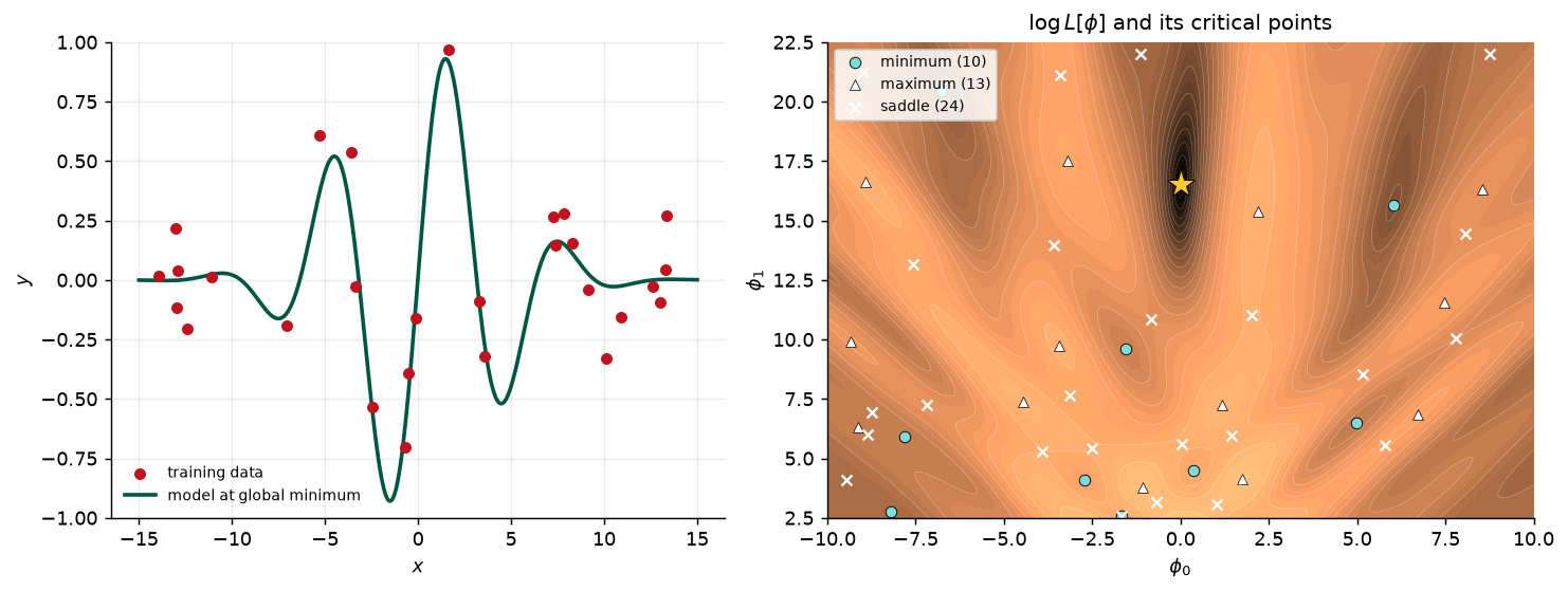
critical points in the window: 10 minima, 13 maxima, 24 saddle points
global minimum: phi = [0.014, 16.518], loss 0.510   (data generated from [0, 16.6])
losses at the other minima: [ 2.16  2.75  3.46  4.49  4.51  5.07  9.52 10.03 11.65]
Ten minima, and only one of them is the answer. The sum of the squared noise in our 28 points is roughly what the global minimum leaves behind, so the global minimum recovers the generating parameters almost exactly. Every other minimum is a qualitatively wrong model that no small change can improve. Also note how much of the map is plateau: where \(|\phi_0|\) is large the Gabor function is nearly zero over the whole dataset, the loss is close to \(\sum_i y_i^2\), and the gradient is close to zero — not because we are near a solution but because nothing we do matters there.
Prince §6.1.3, pp. 81–83; figures on pp. 82–83.
Fig. 8 is Prince’s version of the same surface. At each cyan circle the gradient is zero and the loss increases in every direction, yet we are not at the lowest point; the lowest point, the global minimum, is the gray circle, with a loss of 0.64 on his data. Panels (b)–(f) show the model at five of the minima, and in every one of them no small change improves the fit.
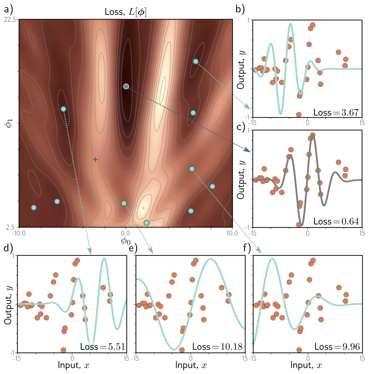
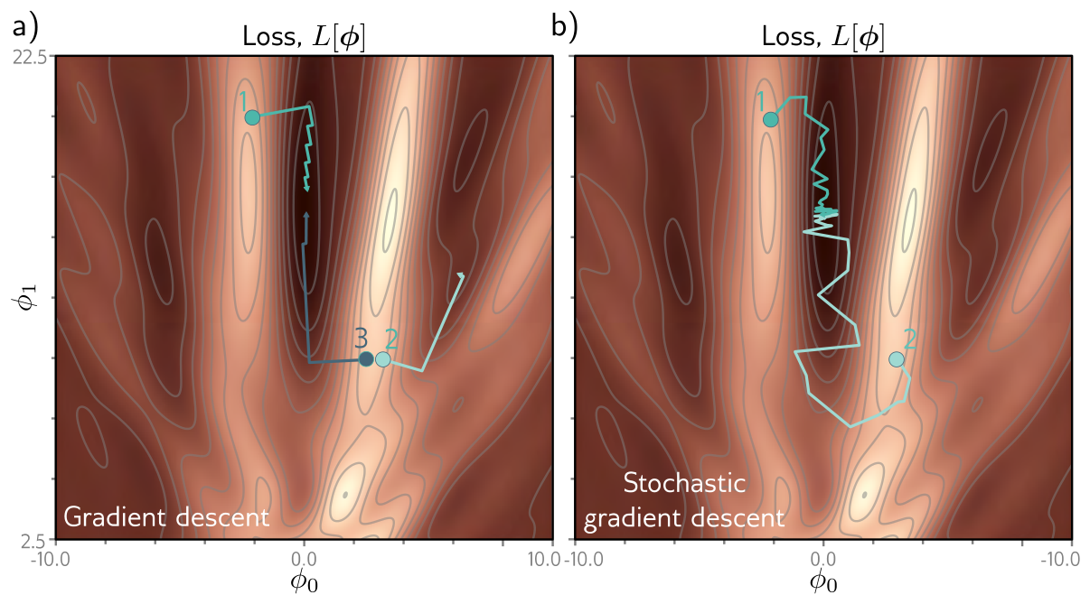
Start somewhere at random and walk downhill, and nothing guarantees you arrive at the global minimum (fig. 9a). Prince puts it bluntly: it is equally or even more likely that the algorithm terminates in one of the local minima, and there is no way of knowing whether a better solution exists elsewhere.
“Equally or even more likely” can be measured. Below, gradient descent starts from every point of the same 41 × 41 grid, and we record where each run ends.
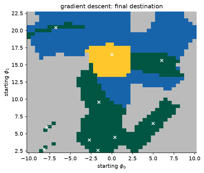
global minimum           5.2%
other local minimum     21.9%
plateau                 43.2%
still moving            29.7%
Only about one start in twenty finds the global minimum, while one in five settles confidently into one of the nine wrong minima — so on this surface, “equally or even more likely” is an understatement by a factor of four. Most of the rest never really get going: over two in five began on a plateau, where the gradient is too small to move the parameters anywhere in 3,000 steps, and the blue region is still creeping along shallow valley floors when the budget runs out. With two parameters we could escape this by brute force — search the whole grid, or restart from many points and keep the best — but a network has millions of parameters, and neither strategy scales. We can find a minimum; we cannot tell whether it is the global one, or even a good one.
The Gabor model is chosen because it is drawable, not because it is typical. Prince’s footnote on p. 91 previews Chapter 20: in practice deep networks are surprisingly easy to train, and whether local minima and saddle points are a real obstacle in very high dimensions is a research question in its own right. Treat this section as the vocabulary for failures, not a forecast of them.
Prince §6.1.3, p. 83.
The surface also contains saddle points — the blue cross in fig. 8 is one — where the gradient is zero but the function increases in some directions and decreases in others. Unless the parameters sit exactly at the saddle, gradient descent will eventually escape downhill. The trouble is the word “eventually”. Near a saddle the surface is flat, so it is hard to be sure that training has not converged, and a stopping rule of the form “terminate when the gradient is small” can stop us at the saddle.
The simplest function with this behaviour makes the point vividly: \(L[\phi_0, \phi_1] = \tfrac{1}{4}\phi_0^4 - \tfrac{1}{2}\phi_0^2 + \tfrac{1}{2}\phi_1^2\) has a saddle at the origin and minima at \((\pm 1, 0)\).
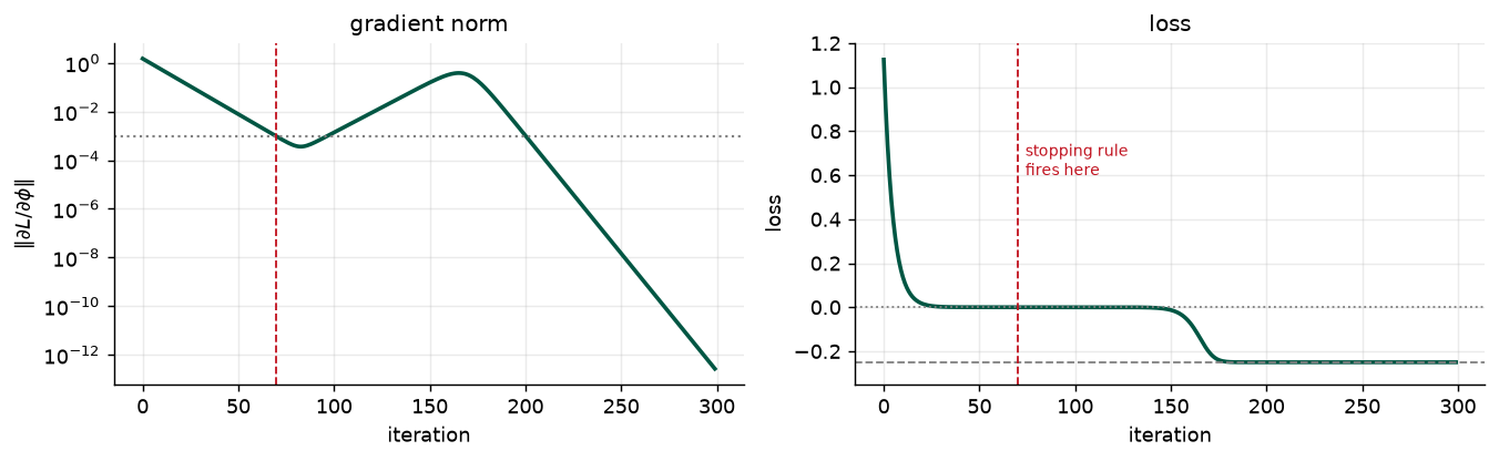
the gradient norm first drops below 1e-3 at iteration 70: phi = [1. 0.] at the end, but at iteration 70 the loss was 4.39e-07 (saddle value 0)
smallest gradient norm on the way past the saddle: 3.6e-04
final loss: -0.2500   (true minimum -0.25)
A starting offset of \(10^{-7}\) is not contrived: in floating point, some tiny component along the escape direction is almost always present, which is why gradient descent rarely gets permanently stuck on a saddle. It gets slow. In a space of millions of parameters, Chapter 20 will argue, saddle points vastly outnumber local minima, and the long plateaus they create are a more realistic threat than being trapped.
Prince §6.2, pp. 83–85.
Gradient descent has a deeper problem than slowness: its final destination is completely determined by its starting point (fig. 10 is a map of exactly that dependence). Stochastic gradient descent (SGD) tries to loosen this by adding noise to the gradient at each step. On average the solution still moves downhill, but at any single iteration the chosen direction need not be the steepest descent — it need not be downhill at all. Moving temporarily uphill is what allows the parameters to jump from one valley of the loss to another (fig. 9b).
Prince §6.2.1, p. 85; figure on p. 84.
The mechanism for the noise is almost embarrassingly simple, and it follows directly from eq. 6. At each iteration, choose a random subset of the training data — a minibatch, or batch for short — and compute the gradient from those examples alone. The update at iteration \(t\) is
\[ \boldsymbol{\phi}_{t+1} \longleftarrow \boldsymbol{\phi}_t - \alpha \cdot \sum_{i \in \mathcal{B}_t} \frac{\partial \ell_i[\boldsymbol{\phi}_t]}{\partial \boldsymbol{\phi}}, \tag{11}\]
where \(\mathcal{B}_t\) holds the indices of the examples in the current batch and \(\ell_i\) is the loss of the \(i\)th example. As before, \(\alpha\) is the learning rate, chosen at the start and independent of the local shape of the function; together with the gradient magnitude it determines how far each step goes.
Batches are usually drawn without replacement. The algorithm works through the training examples until every one has been used, then starts again from the full set. One complete pass is an epoch. A batch can be as small as a single example or as large as the whole dataset; the second case is full-batch gradient descent, which is identical to the ordinary, non-stochastic gradient descent of eq. 3.
There is a second way to read eq. 11, and it is the one fig. 12 illustrates. The loss depends on both the model and the data, so each batch defines its own loss function. SGD can then be seen as performing ordinary, deterministic gradient descent on a loss function that changes at every iteration. Panels (b)–(d) show three batches of three examples, three different surfaces, and three different steps from the same point — and in panel (d), a step that is downhill on its batch’s surface but uphill on the full one.
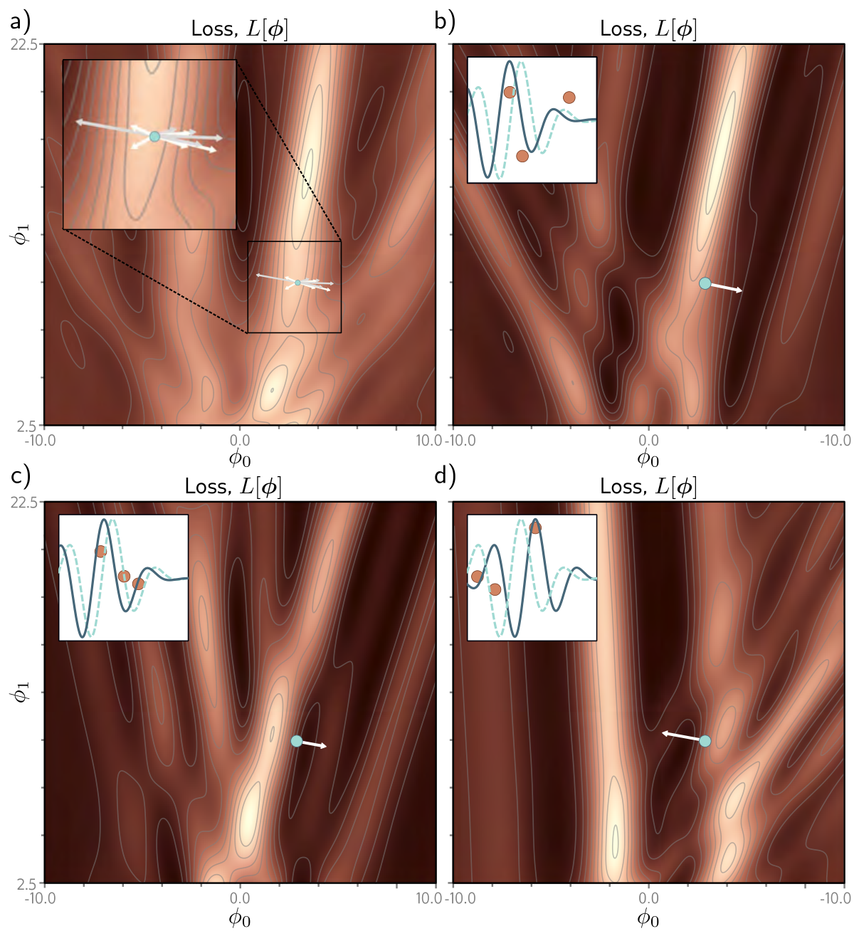
Despite that variability, the expected loss and the expected gradient at any point are the same as for full-batch descent: averaged over the possible batches, a batch of \(B\) examples contributes on average \(B/I\) of the full gradient. Both claims are easy to check by sampling.
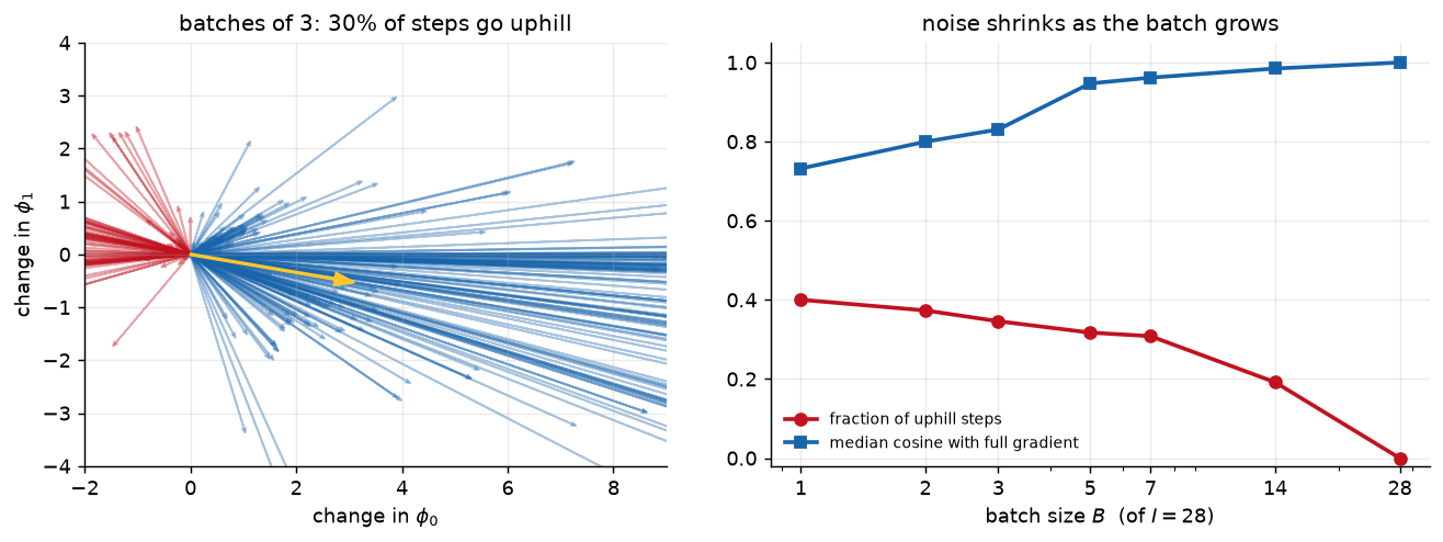
   B   uphill  median cos    |mean(I/B * batch grad) - full| / |full|
   1    40.0%       0.732                                       0.082
   2    37.3%       0.800                                       0.009
   3    34.6%       0.831                                       0.011
   5    31.7%       0.947                                       0.004
   7    30.8%       0.962                                       0.017
  14    19.2%       0.985                                       0.016
  28     0.0%       1.000                                       0.000
The last column is the unbiasedness claim: averaged over 4,000 batches and rescaled by \(I/B\), the batch gradient matches the full gradient to within sampling error at every batch size. The middle columns are the noise. With a single example per batch, more than a third of all steps are uphill on the full loss; even at half the dataset, one in five is.
Prince §6.2.2, pp. 85–86.
Prince lists the attractions of SGD, and each is worth stating precisely.
Property 4 carries the words “in principle”, and it is worth testing them honestly. The comparison has a trap. SGD is usually run with larger steps than gradient descent, and a larger step can carry the parameters over a ridge by itself, noise or no noise. So below, each SGD run is paired with a full-batch run that uses the same per-example step size, the same schedule, and the same number of updates. Any difference between them is due to the noise alone.
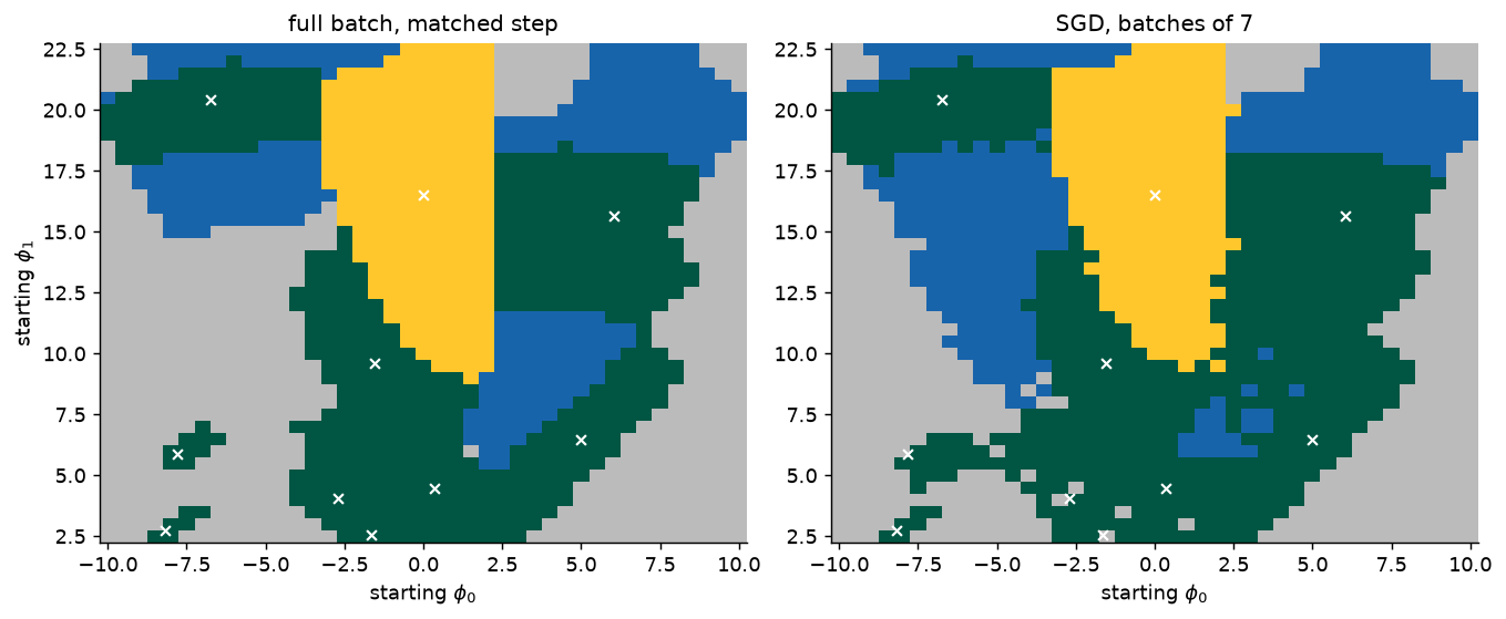
outcome                 GD, fixed small step  GD, matched step     SGD
global minimum                          5.2%             14.2%   14.0%
other local minimum                    21.9%             32.9%   37.7%
plateau                                43.2%             35.5%   28.4%
still moving                           29.7%             17.4%   19.9%
This is a useful result precisely because it is not the one the textbook picture invites. Larger steps nearly triple the number of starts that reach the global minimum; the noise on top of them changes that count by a fraction of a percentage point. Where the noise does earn its keep is property 5: SGD strands noticeably fewer runs on the plateau, because even where the full gradient vanishes, some batches do not. But follow those rescued runs and most of them roll into a wrong minimum — escaping a flat region is not the same as finding a good one. On a two-parameter surface with deep, widely separated valleys, 28 examples simply cannot generate enough noise to climb out of a wrong valley that full-batch descent has settled into. Whether the same is true of a network with millions of parameters is a different and much more interesting question, and it is the one Chapters 9 and 20 take up.
Prince §6.2.2, p. 86; chapter notes, p. 93.
SGD does not “converge” in the classical sense: near any minimum, every batch still pulls in a slightly different direction, so with a fixed \(\alpha\) the parameters keep jittering. The hope is that close to the global minimum all the examples are well described, every batch gradient is small, and the jitter dies down on its own.
In practice SGD is almost always run with a learning rate schedule. The standard one starts \(\alpha\) high and divides it by a constant factor every \(N\) epochs. The logic has two phases. Early in training we want to explore — jump from valley to valley until we find a sensible region. Later we are roughly in the right place and want to fine-tune, so smaller steps make smaller changes.
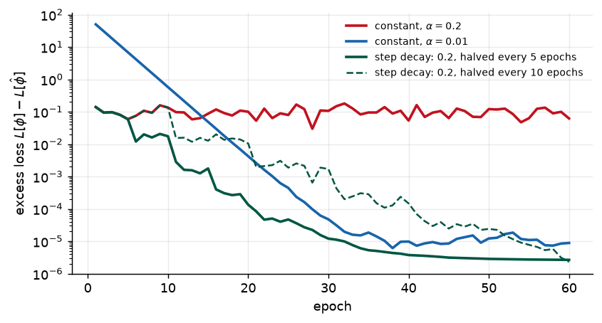
schedule                                        epoch 5   epoch 20   epoch 60   epochs behind alpha = 0.01
constant, alpha = 0.2                          5.91e-02   1.00e-01   6.21e-02                           46
constant, alpha = 0.01                         6.88e+00   4.24e-03   8.89e-06                            0
step decay: 0.2, halved every 5 epochs         5.91e-02   1.35e-04   2.67e-06                            0
step decay: 0.2, halved every 10 epochs        5.91e-02   1.05e-02   2.32e-06                           33
The chapter notes add one refinement for adaptive methods like Adam (below): learning rate warm-up, which starts with a small rate and increases it over the first few thousand iterations, because the running statistics those methods depend on are unreliable until enough gradients have been seen. Modern recipes typically combine both: a short warm-up, then a decay.
Prince §6.3, p. 86; figure on p. 87.
A common modification to SGD adds a momentum term. Rather than stepping along the current batch gradient, step along a weighted combination of that gradient and the direction moved at the previous step:
\[ \begin{aligned} \mathbf{m}_{t+1} &\longleftarrow \beta \cdot \mathbf{m}_t + (1 - \beta) \sum_{i \in \mathcal{B}_t} \frac{\partial \ell_i[\boldsymbol{\phi}_t]}{\partial \boldsymbol{\phi}} \\ \boldsymbol{\phi}_{t+1} &\longleftarrow \boldsymbol{\phi}_t - \alpha \cdot \mathbf{m}_{t+1}, \end{aligned} \tag{12}\]
where \(\mathbf{m}_t\) is the momentum that drives the update at iteration \(t\), \(\beta \in [0, 1)\) controls how strongly the gradient is smoothed over time, and \(\alpha\) is the learning rate.
Because \(\mathbf{m}\) is defined recursively, each step is an infinite weighted sum of all previous gradients, with weights that shrink the further back we go (problem 6.10 asks for the weights). That has a simple consequence. Where successive gradients agree — along the floor of a long valley — they add up and the effective step grows. Where they alternate — across the valley, from wall to wall — they cancel. The result is a smoother trajectory with much less oscillation (fig. 16).
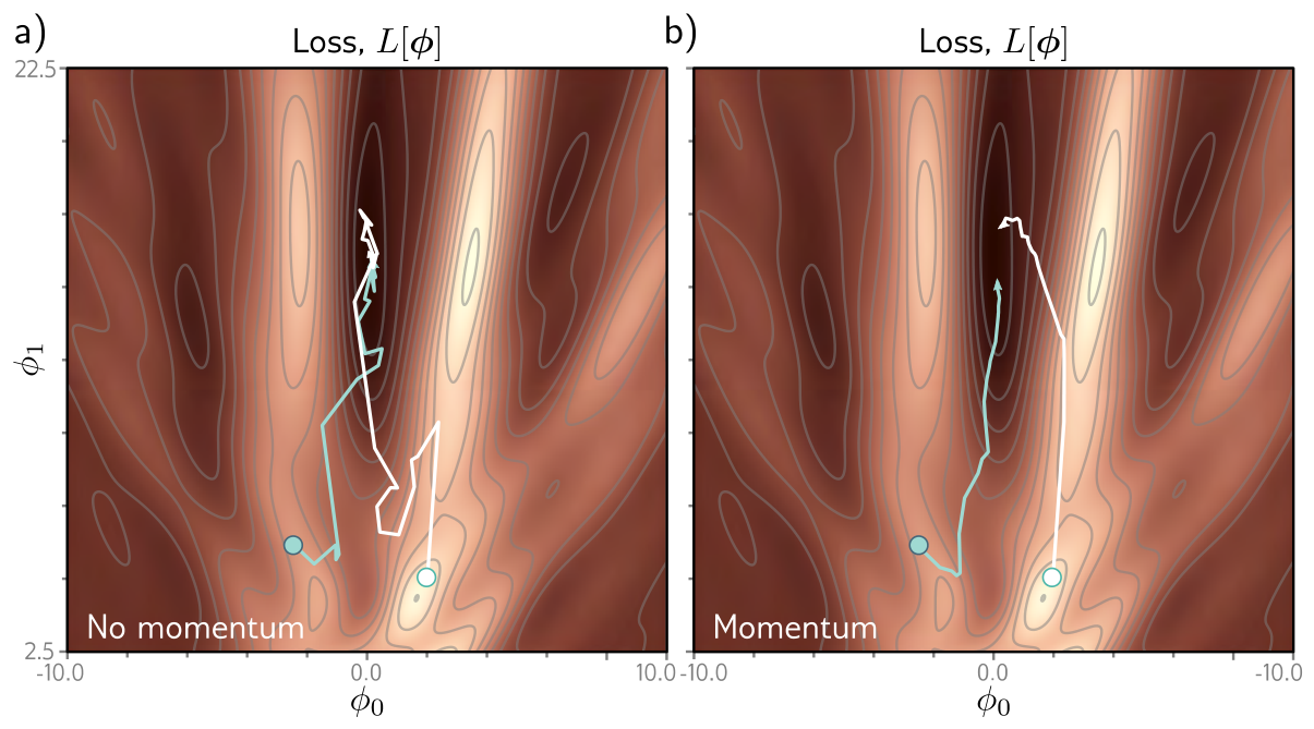
The deterministic version of this is the clearest. Take a quadratic bowl with condition number 100, so gradient descent faces exactly the dilemma of fig. 4, and give gradient descent, momentum, and Nesterov momentum (next subsection) each the best hyperparameters from a common grid.
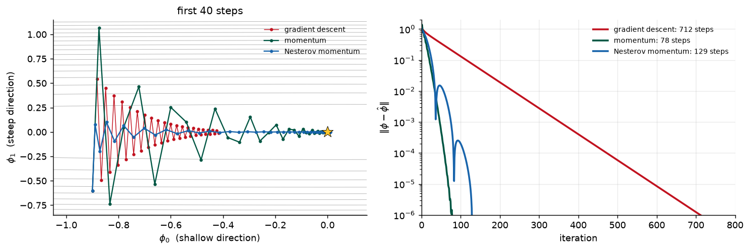
method                 alpha   beta  steps to 1e-6
gradient descent       0.191   0.00            712
momentum               0.927   0.70             78
Nesterov momentum      0.751   0.85            129

stability limit of plain gradient descent, 2 / lambda_max = 0.200
Two numbers carry the lesson. Momentum is roughly nine times faster than the best gradient descent, and it gets there with a learning rate several times above gradient descent’s stability limit — a step that would diverge without the momentum term. Theory predicts this: on a quadratic, the iterations gradient descent needs grow with the condition number \(\kappa\), while momentum with well-chosen coefficients needs a number that grows only with \(\sqrt{\kappa}\). At \(\kappa = 100\) that is the difference between hundreds of steps and tens.
Prince §6.3.1, pp. 86–88; figure on p. 87.
The momentum term is a coarse prediction of where the algorithm is about to go. Nesterov accelerated momentum takes that prediction seriously and measures the gradient there, at the look-ahead point, instead of at the current one:
\[ \begin{aligned} \mathbf{m}_{t+1} &\longleftarrow \beta \cdot \mathbf{m}_t + (1 - \beta) \sum_{i \in \mathcal{B}_t} \frac{\partial \ell_i[\boldsymbol{\phi}_t - \alpha \cdot \mathbf{m}_t]}{\partial \boldsymbol{\phi}} \\ \boldsymbol{\phi}_{t+1} &\longleftarrow \boldsymbol{\phi}_t - \alpha \cdot \mathbf{m}_{t+1}. \end{aligned} \tag{13}\]
Fig. 18 shows the difference geometrically. Ordinary momentum, at point 1, measures the gradient there, steps along it to point 2, and then adds the momentum term to arrive at point 3. Nesterov momentum applies the momentum term first, moving from point 1 to point 4, then measures the gradient at 4 and corrects to point 5. One way to read it: the gradient now corrects the path that momentum alone would have taken, rather than being added to it blindly.
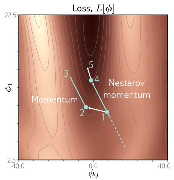
On our quadratic, Nesterov’s grid-best settings needed more steps than ordinary momentum’s — not a contradiction. For a quadratic, ordinary (“heavy-ball”) momentum with tuned coefficients is already optimal; Nesterov’s advantage is a convergence guarantee for general smooth convex functions where heavy-ball momentum can fail, plus a well-documented robustness in deep learning practice (Sutskever et al. 2013). Both beat plain gradient descent by a wide margin.
Prince §6.4, pp. 88–90; figure on p. 89.
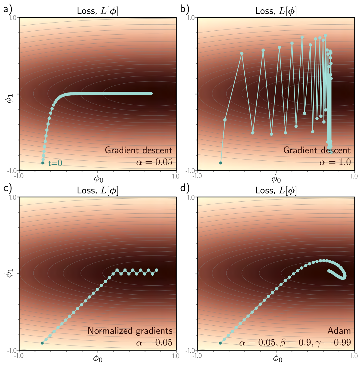
Gradient descent with a fixed step size has an undesirable property that the condition number made concrete: it makes large adjustments to parameters with large gradients, where perhaps it should be cautious, and small adjustments to parameters with small gradients, where perhaps it should explore. When the loss is much steeper in one direction than another, no single learning rate both makes good progress in every direction and is stable (fig. 19a–b).
A direct fix is to normalize the gradient so that every coordinate moves the same distance. Measure the gradient \(\mathbf{m}_{t+1}\) and the pointwise squared gradient \(\mathbf{v}_{t+1}\),
\[ \mathbf{m}_{t+1} \longleftarrow \frac{\partial L[\boldsymbol{\phi}_t]}{\partial \boldsymbol{\phi}}, \qquad \mathbf{v}_{t+1} \longleftarrow \left( \frac{\partial L[\boldsymbol{\phi}_t]}{\partial \boldsymbol{\phi}} \right)^2, \tag{14}\]
and update with
\[ \boldsymbol{\phi}_{t+1} \longleftarrow \boldsymbol{\phi}_t - \alpha \cdot \frac{\mathbf{m}_{t+1}}{\sqrt{\mathbf{v}_{t+1}} + \epsilon}, \tag{15}\]
where the square root and division are taken element by element, and the small constant \(\epsilon\) prevents division by zero. Dividing the gradient by its own magnitude leaves only its sign in each coordinate, so every parameter moves a fixed distance \(\alpha\), downhill. That makes good progress in all directions — but it can never settle unless it happens to land exactly on the minimum. Instead it rattles back and forth around it (fig. 19c).
Adaptive moment estimation, or Adam, keeps the normalization and adds momentum to both statistics:
\[ \begin{aligned} \mathbf{m}_{t+1} &\longleftarrow \beta \cdot \mathbf{m}_t + (1 - \beta) \frac{\partial L[\boldsymbol{\phi}_t]}{\partial \boldsymbol{\phi}} \\ \mathbf{v}_{t+1} &\longleftarrow \gamma \cdot \mathbf{v}_t + (1 - \gamma) \left( \frac{\partial L[\boldsymbol{\phi}_t]}{\partial \boldsymbol{\phi}} \right)^2, \end{aligned} \tag{16}\]
with momentum coefficients \(\beta\) and \(\gamma\) for the two statistics. Each is now a weighted average over the history of the gradient and of its square. That creates one problem at the start: the averages begin at zero, so for the first few iterations both are unrealistically small. Adam corrects them,
\[ \tilde{\mathbf{m}}_{t+1} \longleftarrow \frac{\mathbf{m}_{t+1}}{1 - \beta^{t+1}}, \qquad \tilde{\mathbf{v}}_{t+1} \longleftarrow \frac{\mathbf{v}_{t+1}}{1 - \gamma^{t+1}}, \tag{17}\]
and since \(\beta, \gamma \in [0, 1)\) the powers shrink every step, the denominators approach one, and the correction fades out. The update uses the corrected statistics:
\[ \boldsymbol{\phi}_{t+1} \longleftarrow \boldsymbol{\phi}_t - \alpha \cdot \frac{\tilde{\mathbf{m}}_{t+1}}{\sqrt{\tilde{\mathbf{v}}_{t+1}} + \epsilon}. \tag{18}\]
The result converges to the minimum and still makes good progress in every direction of parameter space (fig. 19d). In practice Adam is run stochastically, with both statistics accumulated from batches,
\[ \begin{aligned} \mathbf{m}_{t+1} &\longleftarrow \beta \cdot \mathbf{m}_t + (1 - \beta) \sum_{i \in \mathcal{B}_t} \frac{\partial \ell_i[\boldsymbol{\phi}_t]}{\partial \boldsymbol{\phi}} \\ \mathbf{v}_{t+1} &\longleftarrow \gamma \cdot \mathbf{v}_t + (1 - \gamma) \left( \sum_{i \in \mathcal{B}_t} \frac{\partial \ell_i[\boldsymbol{\phi}_t]}{\partial \boldsymbol{\phi}} \right)^2, \end{aligned} \tag{19}\]
so the trajectory is noisy, like every other method in this chapter.
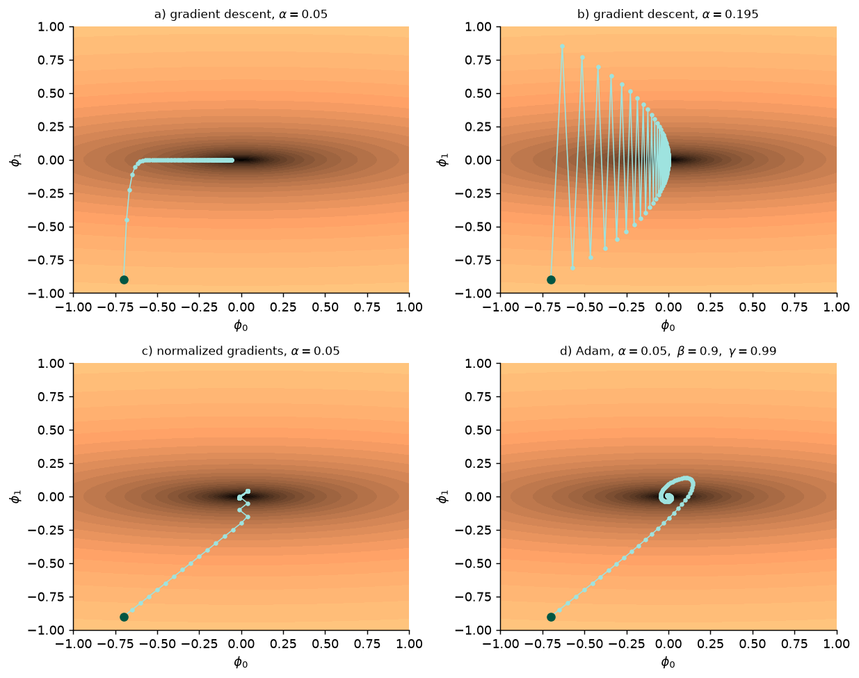
method                                               |phi| after 20         50        100
a) gradient descent, alpha = 0.05                          4.22e-01   1.97e-01   5.57e-02
b) gradient descent, alpha = 0.195                         3.35e-01   6.94e-02   5.33e-03
c) normalized gradients, alpha = 0.05                      1.62e-02   1.62e-02   1.62e-02
d) Adam, alpha = 0.05, beta = 0.9, gamma = 0.99            1.03e-01   4.62e-02   4.58e-03
Read the columns left to right. The normalized-gradient method gets close fastest and then stops improving at all, frozen at a distance set by \(\alpha\). Gradient descent with the safe step is still far away after 100 steps. Adam ends closest of the four — narrowly ahead of panel (b), which only does well because its step was tuned to sit just inside this particular bowl’s stability limit. Adam reached that point with the same cautious \(\alpha = 0.05\) that crippled panel (a), and without knowing anything about the curvature. Notice also what eq. 16 becomes with \(\beta = \gamma = 0\): the statistics are just the current gradient and its square, and Adam is the normalized-gradient method of panel (c). Momentum on the squared gradient is what turns a fixed-size rattle into convergence.
Three more claims from the section can be checked directly: what the bias correction does, that our six lines agree with PyTorch’s Adam, and the promise that Adam is less sensitive to the learning rate.
bias correction, equation (6.16), with PyTorch's defaults beta = 0.9, gamma = 0.999
a constant gradient g = 1 gives these running averages before and after correction:

   t      m_t    m~_t       v_t    v~_t   update without correction
   1   0.1000     1.0    0.0010     1.0                       3.162 x alpha
   2   0.1900     1.0    0.0020     1.0                       4.250 x alpha
   3   0.2710     1.0    0.0030     1.0                       4.950 x alpha
   4   0.3439     1.0    0.0040     1.0                       5.442 x alpha
   5   0.4095     1.0    0.0050     1.0                       5.797 x alpha

our equations (6.15)-(6.17) vs torch.optim.Adam over 200 steps: max difference 1.8e-15

multiply the same loss by k, keep every hyperparameter fixed, run 300 steps:
       k     SGD (lr 0.15): |w - w*|    Adam (lr 0.05): |w - w*|
       1                    9.51e-03                    8.20e-06
    1000                         nan                    8.20e-06
The table holds a small surprise. Each statistic on its own is indeed far too small at the start — \(\mathbf{m}\) by a factor of ten, \(\mathbf{v}\) by a factor of a thousand — just as Prince says. But they enter the update as a ratio, and the two biases do not cancel: dividing by \(\sqrt{\mathbf{v}}\) over-corrects, so an uncorrected first step would be more than three times larger than intended, at exactly the moment the statistics are least trustworthy. The correction makes the first step the full \(\alpha\) in every coordinate; warm-up, from the previous section, guards against the same early instability from the other side. The second check confirms there is nothing hidden in PyTorch’s implementation — it is eq. 18 to machine precision. The third is the practical point. Scaling the loss by 1,000 scales every gradient by 1,000, so SGD’s carefully chosen learning rate is suddenly 1,000 times too large and the run blows up. Adam divides each gradient by its own running magnitude, so the scale cancels and the trajectory is unchanged.
That invariance is why the section closes the way it does. Chapter 7 will show that gradient magnitudes in a network depend on a parameter’s depth, and Adam compensates for that tendency, balancing the size of the updates across layers. It is also less sensitive to the initial learning rate, because it avoids the failure modes of fig. 19a–b by construction, and so it rarely needs an elaborate schedule. These are the reasons it is the default optimizer in most of deep learning.
The chapter notes (p. 93) trace the lineage. AdaGrad gave each parameter its own learning rate by dividing by the cumulative squared gradient, which made the rates shrink forever and could halt learning before the minimum. RMSProp and AdaDelta replaced the cumulative sum with a running average — eq. 16’s \(\mathbf{v}\) without the bias correction. Adam combined that with momentum on \(\mathbf{m}\) (Kingma and Ba 2015). Its original convergence proof turned out to have a hole (Reddi, Kale, and Kumar 2018), and AdamW fixed the way Adam interacts with \(L_2\) regularization (Loshchilov and Hutter 2019), which is a Chapter 9 topic; AdamW is the variant most large models are actually trained with. Whether well-tuned SGD with momentum generalizes better than Adam has been argued for years (Wilson et al. 2017); the current consensus is that the gap mostly closes when Adam’s hyperparameters are searched as carefully as SGD’s.
Prince §6.5, p. 91.
Every choice made in this chapter — the algorithm, the batch size, the learning rate and its schedule, the momentum coefficients — is a hyperparameter of the training algorithm. These are distinct from the model’s parameters \(\boldsymbol{\phi}\), which training sets, and from the architectural hyperparameters of Week 4, which fix the family of functions; yet they directly affect the model you end up with. Choosing them is, in Prince’s words, more art than science. The usual approach is to train many models with different settings and keep the best, which is called hyperparameter search and is a topic for Chapter 8.
| Hyperparameter | Typical starting point | What goes wrong if it is off |
|---|---|---|
| algorithm | Adam (or AdamW) | — |
| learning rate \(\alpha\) | \(10^{-3}\) for Adam; \(10^{-2}\)–\(10^{-1}\) for SGD | too high diverges; too low stalls |
| batch size \(B\) | 32–256 | too small is noisy and slow per epoch; too large wastes compute per step |
| momentum \(\beta\) | 0.9 | too close to 1 overshoots and oscillates |
| Adam \(\gamma\) | 0.999 | too small makes the normalization noisy |
| schedule | warm-up, then step or cosine decay | none at all leaves SGD at its noise floor |
Ours; UDL notebooks 6.1–6.5.
Every algorithm in this chapter is one line of PyTorch, and the training loop around it never changes: zero the gradients, compute the loss on a batch, backpropagate, step.
| Algorithm | Equation | PyTorch |
|---|---|---|
| SGD | eq. 11 | torch.optim.SGD(params, lr) |
| SGD with momentum | eq. 12 | torch.optim.SGD(params, lr, momentum=0.9) |
| SGD with Nesterov momentum | eq. 13 | torch.optim.SGD(params, lr, momentum=0.9, nesterov=True) |
| Adam | eq. 19 | torch.optim.Adam(params, lr, betas=(0.9, 0.999)) |
| step-decay schedule | — | torch.optim.lr_scheduler.StepLR(opt, step_size, gamma) |
One trap is worth a cell of its own. PyTorch’s momentum is not eq. 12. It accumulates \(\mathbf{b}_{t+1} = \beta \mathbf{b}_t + \mathbf{g}_t\), with no \((1 - \beta)\) on the gradient, and steps by the learning rate times \(\mathbf{b}\). The two agree exactly when PyTorch’s learning rate is set to \(\alpha(1 - \beta)\).
Prince alpha = 0.1, beta = 0.9  <=>  torch.optim.SGD(lr = 0.010, momentum = 0.9)
max difference over 200 steps: 8.9e-16

so torch.optim.SGD(lr = 0.05, momentum = 0.9) is Prince's alpha = 0.50:
adding momentum=0.9 to an SGD run multiplies its effective step size by ten.
The practical consequence: switching on momentum=0.9 in PyTorch without touching lr is not “the same step size plus smoothing” — it makes the effective step ten times larger. Sometimes that is exactly why momentum seemed to help.
Finally, the three optimizers on a real, if small, network: two hidden layers of 32 ReLU units fitting 256 noisy samples of a smooth curve with batches of 16.
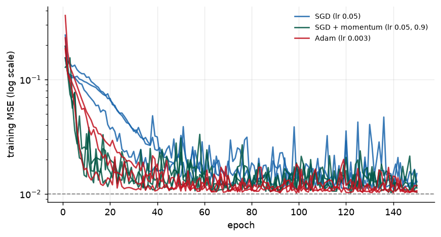
optimizer                         epoch 10  epoch 50  epoch 150   (median of 3 runs)
SGD (lr 0.05)                       0.0944    0.0180     0.0129
SGD + momentum (lr 0.05, 0.9)       0.0246    0.0231     0.0113
Adam (lr 0.003)                     0.0464    0.0112     0.0107
On a problem this small every reasonable optimizer gets there; the differences are in how fast and how smoothly. That is the typical picture, and it is why the choice of optimizer matters most when compute is the binding constraint.
momentum=0.9 multiplies the effective step by ten relative to eq. 12.Prince §6.6, p. 91.
Training was framed as finding the parameters \(\boldsymbol{\phi}\) at the minimum of a loss \(L[\boldsymbol{\phi}]\). Gradient descent measures the gradient of the loss at the current parameters — how the loss changes under a small change to each — and moves in the direction that decreases the loss fastest, repeating until the gradient vanishes. Its step is set either by a fixed learning rate, limited by the steepest curvature of the loss, or by a line search.
For nonlinear models the loss is non-convex. It can have local minima, where gradient descent is trapped, and saddle points, where it can appear to have converged when it has not. Stochastic gradient descent computes each gradient from a random batch of the data, which makes every step cheap and adds noise that, in principle, helps the parameters leave bad regions; it is usually run with a learning rate schedule that explores first and fine-tunes later. Momentum averages the gradient over time, cancelling oscillation across valleys and accelerating progress along them; Nesterov momentum measures the gradient at the point momentum is about to reach. Adam normalizes each parameter’s step by a running estimate of its gradient magnitude and smooths both statistics, which makes good progress in every direction, is insensitive to the scale of the gradients, and is the default optimizer of modern deep learning.
The ideas in this chapter apply to optimizing any model. Nothing in them is specific to neural networks.
Next: every algorithm here assumed the gradient \(\partial L / \partial \boldsymbol{\phi}\) was available. For a deep network it is not obvious how to get it efficiently, and Chapter 7 derives the backpropagation algorithm that computes it. It also addresses the other loose end of this week’s loop — the initial parameters — and shows that without care, gradients in deep networks become vanishingly small or explosively large before optimization even begins.
1. (UDL 6.1 and 6.2) Show that the derivatives of the least squares loss eq. 5 are given by eq. 7. Then find an algebraic expression for the \(2 \times 2\) Hessian of the same loss and prove the loss is convex by showing that both eigenvalues are always positive. (Hint: it is enough to show that the trace and the determinant are both positive; Week 2 has the facts you need.) Check your expression against H_lin in fig. 4.
2. (UDL 6.3 and 6.5*) Compute the derivatives of the Gabor loss eq. 10 with respect to \(\phi_0\) and \(\phi_1\), and verify them against grad_L in the notebook at three points of your choice. Then compute the derivatives of the least squares loss with respect to all ten parameters of the shallow network of Week 3, \[
\mathrm{f}[x, \boldsymbol{\phi}] = \phi_0 + \phi_1 a[\theta_{10} + \theta_{11}x] + \phi_2 a[\theta_{20} + \theta_{21}x] + \phi_3 a[\theta_{30} + \theta_{31}x],
\] thinking carefully about the derivative of the ReLU \(a[\bullet]\). What is it at exactly zero, and does it matter in practice?
3. (UDL 6.4*) The logistic regression model \(Pr(y = 1 \mid x) = \mathrm{sig}[\phi_0 + \phi_1 x]\) assigns a scalar input to one of two classes. (i) Plot \(Pr(y = 1 \mid x)\) for several \((\phi_0, \phi_1)\) and explain what each parameter does. (ii) Using Week 5, what is the right loss? (iii) Compute its derivatives. (iv) Generate ten points from \(\mathcal{N}(-1, 1)\) labelled \(y = 0\) and ten from \(\mathcal{N}(1, 1)\) labelled \(y = 1\), and plot the loss as a heatmap over \((\phi_0, \phi_1)\). (v) Is it convex? How would you prove it?
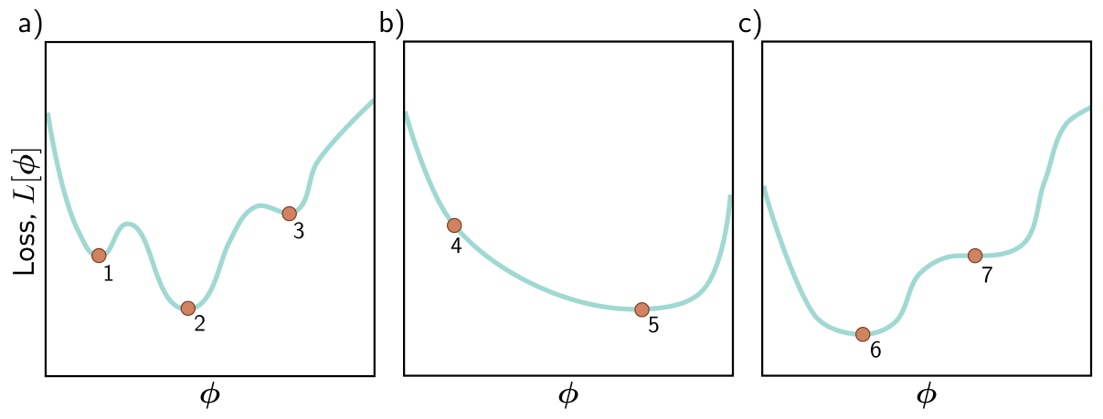
4. (UDL 6.6) Which of the functions in fig. 22 is convex? Justify your answer. Classify each of the points 1–7 as a local minimum, the global minimum, or neither.
5. (UDL 6.7* and 6.8*) The gradient descent path in fig. 3, like path 1 in fig. 9a, turns through a large angle at every step, and with an exact line search the turn is a right angle. Explain why, and propose a fix. Then answer: can non-stochastic gradient descent with a fixed learning rate ever escape a local minimum? Use fig. 4 to sharpen your answer — is there a sense in which a step size above the stability limit “escapes”?
6. (UDL 6.9 and 6.11) We run SGD for 1,000 iterations on a dataset of 100 examples with a batch size of 20. For how many epochs did we train? Separately: what are the dimensions of the Hessian of a model with one million parameters, how many gigabytes would it take to store in 32-bit floating point, and what does that imply for Newton’s method in deep learning?
7. (UDL 6.10) Show that the momentum \(\mathbf{m}_t\) of eq. 12 is an infinite weighted sum of the gradients at previous iterations, and derive the weights. Show they sum to one in the limit. Then use your result to explain the momentum-convention cell: why does PyTorch’s form, without the \((1 - \beta)\), amplify the steady-state step by a factor of \(1/(1 - \beta)\)?
8. A maintenance engineer fits a damped-vibration model to a hammer-tap test on a machine-tool spindle, \(y(t) = A\, e^{-\zeta \omega t} \sin[\omega t]\), by least squares on 400 accelerometer samples, using gradient descent from \(\omega = 100\) rad/s. The true natural frequency is near 900 rad/s. (a) By analogy with the Gabor model, sketch what the loss looks like as a function of \(\omega\) alone and explain why the fit converges to a poor answer. (b) Would SGD help? Use fig. 14 in your answer. (c) Propose a physics-based initialization that makes the optimization easy, and explain why a good starting point is worth more here than a better optimizer.
9. Computational. Starting from fig. 10: (a) replace the fixed learning rate with the golden-section line_search of fig. 3 and recompute the outcome map — does the fraction reaching the global minimum change, and why? (b) In fig. 14, vary the batch size over 1, 2, 4, 7, and 14, keeping the matched full-batch comparison each time. At which batch size, if any, does the noise measurably improve the global-minimum count? (c) Report the plateau fraction for each run and connect it to property 5 of SGD.
10. Computational. Using adam_step from fig. 20: (a) remove the bias correction and plot the first 20 steps against the corrected version — which coordinates are affected, and for how long? (b) Run with \(\beta = \gamma = 0\) and confirm it reproduces panel (c). Prince’s notes (p. 94) remark that SGD is a special case of Adam when \(\beta = \gamma = 0\); reconcile that remark with what you see. (c) Sweep \(\alpha\) over \(10^{-3}\) to \(1\) for gradient descent and for Adam on this bowl, and plot the distance after 100 steps against \(\alpha\) for both. Which method has the wider range of good learning rates?
Every part of this page, mapped to Prince, Understanding Deep Learning (MIT Press, 2024) (Prince 2024). Page numbers are those of the printed book.
| This page | Prince section | Pages | Figures used |
|---|---|---|---|
| What Fitting a Model Means | Ch. 6 opening | 77 | — |
| Gradient Descent | §6.1 | 77–78 | — |
| — Choosing the step: learning rate or line search | §6.1; notes | 78, 92–93 | 6.10 (p. 93) |
| — Linear regression example | §6.1.1 | 78–80 | 6.1 (p. 79) |
| Non-Convex Loss Surfaces | §6.1.2; notes | 80–81, 92 | 6.2 (p. 81), 6.3 (p. 81) |
| — Local minima | §6.1.3 | 81–83 | 6.4 (p. 82), 6.5 (p. 83) |
| — Saddle points | §6.1.3 | 83 | — |
| Stochastic Gradient Descent | §6.2 | 83–85 | 6.5 (p. 83) |
| — Batches and epochs | §6.2.1 | 85 | 6.6 (p. 84) |
| — Properties of stochastic gradient descent | §6.2.2 | 85–86 | — |
| — Learning rate schedules | §6.2.2; notes | 86, 93 | — |
| Momentum | §6.3 | 86 | 6.7 (p. 87) |
| — Nesterov accelerated momentum | §6.3.1 | 86–88 | 6.8 (p. 87) |
| Adam | §6.4; notes | 88–90, 93–94 | 6.9 (p. 89) |
| Training Algorithm Hyperparameters | §6.5 | 91 | — |
| Optimizers in PyTorch | ours; notebooks 6.1–6.5 | — | — |
| Summary | §6.6 | 91 | — |
| Exercises 1–7 | Problems 6.1–6.11 | 94–95 | 6.11 (p. 95) |
Equations on this page correspond to Prince as follows: eq. 1 is his (6.1), eq. 2 is (6.2), eq. 3 is (6.3), eq. 4 is (6.4), eq. 5 is (6.5), eq. 6 is (6.6), eq. 7 is (6.7), eq. 9 is (6.8), eq. 10 is (6.9), eq. 11 is (6.10), eq. 12 is (6.11), eq. 13 is (6.12), eq. 14 is (6.13), eq. 15 is (6.14), eq. 16 is (6.15), eq. 17 is (6.16), eq. 18 is (6.17), eq. 19 is (6.18), and eq. 8 is (6.19). The logistic regression model of exercise 3 is his (6.21)–(6.22), and the shallow network of exercise 2 is (6.23).
Figures 6.1–6.11 are reproduced unaltered from Prince, Understanding Deep Learning (MIT Press, 2024), which is distributed under a Creative Commons CC-BY-NC-ND license, and are used here for non-commercial classroom instruction. All other figures on this page are generated by the code in this week’s notebook.