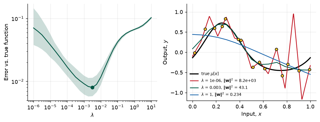
best lambda 3.2e-03: error 0.0080; lambda -> 0: 0.0708; lambda = 10: 0.1031Week 10 · Session 19 · October 27, 2026
Every section below opens with the section number and page range it covers in Prince, Understanding Deep Learning (MIT Press, 2024). Page numbers are those of the printed book. Figures taken from the textbook are captioned with their original figure number and page; figures generated by the code behind this page are ours. A complete cross-reference table appears in Section 9.
By the end of this week you should be able to:
This page shows the figures and results; the Python behind them is not printed here. All of it — every cell, in the order the note uses it — is in a notebook you can open in the browser with nothing to install:
Colab gives you a Python environment with NumPy, matplotlib, and PyTorch already installed. In Colab, run a cell with Shift+Enter. If you prefer to work locally, pip install -r requirements.txt from the course repository gives you the same environment.
Prince, Chapter 9 opening, p. 138.
Chapter 8 measured the gap between training and test performance and traced it to two causes. The model may describe statistical peculiarities of the training set that are not part of the true input–output mapping — that is overfitting. And in regions of the input space with no training examples the model is unconstrained, so what it does there is up to chance. This chapter is about closing the gap.
Prince is careful about the word. Strictly, regularization means adding an explicit term to the loss function that favors certain parameter values. In machine learning the word has come to mean any strategy that improves generalization, and the chapter uses it both ways. Prince starts with the strict sense (§9.1), then shows that the optimizer itself quietly adds regularizing terms we never wrote down (§9.2), and then surveys the heuristics that practitioners rely on (§9.3). The closing picture, fig. 18, sorts all of them into four mechanisms, and it is worth keeping in view from the start: make the function smoother, get more data, combine models, or find a wider minimum.
The passages of Chapter 9 highlighted in the assigned reading get the most space here: what the regularization term is and what it assumes (§9.1), and the practitioner’s toolkit of §9.3 — early stopping, ensembles, dropout, noise and label smoothing, transfer and self-supervised learning, augmentation — with the chapter’s problems 9.1–9.5 worked out where they belong. The derivation of implicit regularization (§9.2) and the Bayesian approach (§9.3.5) are kept shorter; read them for the idea rather than the algebra.
Prince §9.1, pp. 138–139; figure on p. 139.
Training a model \(\mathrm{f}[\mathbf{x}, \boldsymbol{\phi}]\) on pairs \(\{\mathbf{x}_i, y_i\}\) means solving
\[ \hat{\boldsymbol{\phi}} = \underset{\boldsymbol{\phi}}{\operatorname{argmin}} \Big[ L[\boldsymbol{\phi}] \Big] = \underset{\boldsymbol{\phi}}{\operatorname{argmin}} \Big[ \sum_{i=1}^{I} \ell_i[\mathbf{x}_i, y_i] \Big], \tag{1}\]
where each term \(\ell_i\) measures the mismatch between the prediction and the target. To bias the solution toward parameters we prefer, add a term:
\[ \hat{\boldsymbol{\phi}} = \underset{\boldsymbol{\phi}}{\operatorname{argmin}} \Big[ \sum_{i=1}^{I} \ell_i[\mathbf{x}_i, y_i] + \lambda \cdot g[\boldsymbol{\phi}] \Big]. \tag{2}\]
The function \(g[\boldsymbol{\phi}]\) returns a larger scalar for parameters we like less, and \(\lambda > 0\) sets how much the penalty counts against the data term. The minima of the regularized loss are generally not those of the original, so training ends somewhere else. fig. 1 shows the effect on the Gabor loss from Week 6: a bowl-shaped penalty centered on the origin is added to the loss surface, the sum has fewer local minima, and the global minimum has moved.
Three things to notice about eq. 2 before going further.
weight_decay) you read in a paper written for one convention does not transfer to the other without rescaling.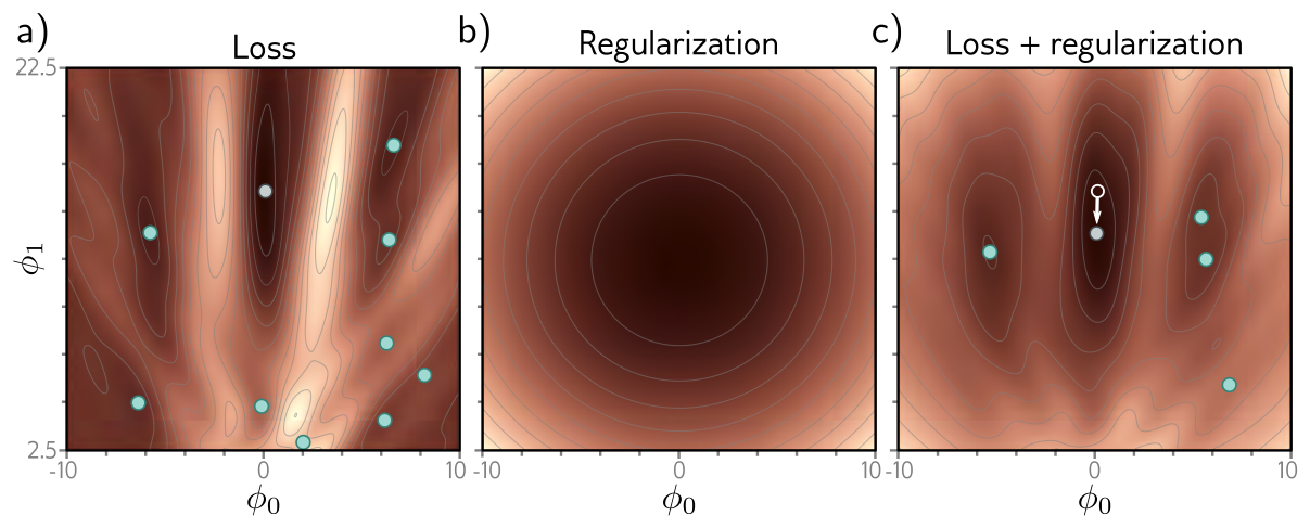
Prince §9.1.1, pp. 139–140.
Week 5 built every loss from the maximum likelihood criterion,
\[ \hat{\boldsymbol{\phi}} = \underset{\boldsymbol{\phi}}{\operatorname{argmax}} \Big[ \prod_{i=1}^{I} Pr(y_i \mid \mathbf{x}_i, \boldsymbol{\phi}) \Big]. \tag{3}\]
A regularizer has a natural reading in that language: it is a prior \(Pr(\boldsymbol{\phi})\), what we believe about the parameters before seeing any data. Multiplying the likelihood by the prior gives the maximum a posteriori or MAP criterion,
\[ \hat{\boldsymbol{\phi}} = \underset{\boldsymbol{\phi}}{\operatorname{argmax}} \Big[ \prod_{i=1}^{I} Pr(y_i \mid \mathbf{x}_i, \boldsymbol{\phi})\, Pr(\boldsymbol{\phi}) \Big]. \tag{4}\]
Take the negative log, as in Week 5. The log of a product is a sum of logs, so
\[ -\log\Big[\prod_{i=1}^{I} Pr(y_i \mid \mathbf{x}_i, \boldsymbol{\phi})\, Pr(\boldsymbol{\phi})\Big] = \underbrace{\sum_{i=1}^{I} -\log Pr(y_i \mid \mathbf{x}_i, \boldsymbol{\phi})}_{\sum_i \ell_i[\mathbf{x}_i, y_i]} \; \underbrace{- \log Pr(\boldsymbol{\phi})}_{\lambda \cdot g[\boldsymbol{\phi}]}, \tag{5}\]
and the regularized loss of eq. 2 appears with \(\lambda \cdot g[\boldsymbol{\phi}] = -\log Pr(\boldsymbol{\phi})\). Every penalty is a prior and every prior is a penalty. The dictionary runs both ways, and it tells you what a given regularizer is assuming: a penalty that grows with \(|\phi_j|\) is the statement “before seeing data, I believe large parameters are improbable.”
Suppose each parameter independently has a zero-mean normal prior with variance \(\sigma^2_\phi\), \(Pr(\boldsymbol{\phi}) = \prod_{j} \mathrm{Norm}_{\phi_j}[0, \sigma^2_\phi]\). Its negative log is \[ -\log Pr(\boldsymbol{\phi}) = \sum_j \Big[ \tfrac{1}{2}\log(2\pi\sigma^2_\phi) + \frac{\phi_j^2}{2\sigma^2_\phi} \Big] = \frac{1}{2\sigma^2_\phi} \sum_j \phi_j^2 + \text{const}. \tag{6}\] The constant does not depend on \(\boldsymbol{\phi}\) and drops out of the argmin, leaving exactly the L2 term of eq. 8 with \[ \lambda = \frac{1}{2\sigma^2_\phi}. \tag{7}\] So the regularization strength is the prior’s tightness: a prior that only believes in small parameters (small \(\sigma^2_\phi\)) is a large \(\lambda\), and a vague prior (\(\sigma^2_\phi \to \infty\)) is no regularization at all. The same calculation with a Laplace prior, \(Pr(\phi_j) \propto e^{-|\phi_j|/b}\), gives the L1 penalty \(\sum_j |\phi_j| / b\) of the chapter notes, which pushes some parameters to exactly zero.
Prince §9.1.2, pp. 140–141; figure on p. 141.
Neural networks are used for so many things that the prior can only express very generic preferences. By far the most common is the L2 norm, which penalizes the sum of the squared parameters:
\[ \hat{\boldsymbol{\phi}} = \underset{\boldsymbol{\phi}}{\operatorname{argmin}} \Big[ \sum_{i=1}^{I} \ell_i[\mathbf{x}_i, y_i] + \lambda \sum_j \phi_j^2 \Big]. \tag{8}\]
Other names for the same thing are Tikhonov regularization, ridge regression, and, for weight matrices, Frobenius norm regularization (the Frobenius norm of a matrix is the square root of the sum of its squared entries, so penalizing it squared is the same sum). As the callout above showed, it is the normal prior with \(\lambda = 1/(2\sigma^2_\phi)\).
Weights, not biases. For networks the penalty is normally applied to the weights \(\boldsymbol{\Omega}_k\) and not the biases \(\boldsymbol{\beta}_k\), and is then called a weight decay term. The reason is what each kind of parameter does. A weight multiplies an activation, so its size sets how steeply the function can change; a bias only shifts where a ReLU’s joint sits or where the output is centred. Shrinking biases toward zero would not make the function smoother, it would just drag every joint toward the origin and the output toward zero — a preference with no justification.
What the gradient sees (problem 9.2). Adding \(\lambda\sum_j \phi_j^2\) to the loss adds \(2\lambda\phi_j\) to every component of the gradient: \[ \frac{\partial}{\partial \boldsymbol{\phi}} \Big[ L[\boldsymbol{\phi}] + \lambda \sum_j \phi_j^2 \Big] = \frac{\partial L}{\partial \boldsymbol{\phi}} + 2\lambda\boldsymbol{\phi}, \tag{9}\] so a gradient descent step becomes \[ \boldsymbol{\phi} \longleftarrow \boldsymbol{\phi} - \alpha\Big(\frac{\partial L}{\partial \boldsymbol{\phi}} + 2\lambda\boldsymbol{\phi}\Big) = (1 - 2\alpha\lambda)\,\boldsymbol{\phi} - \alpha\frac{\partial L}{\partial \boldsymbol{\phi}}. \tag{10}\] Every iteration first multiplies the parameters by a number slightly below one and then takes the usual step. That is where the name weight decay comes from, and eq. 10 is problem 9.5 read backwards: the decay update \(\boldsymbol{\phi} \leftarrow (1 - \lambda')\boldsymbol{\phi} - \alpha\,\partial L/\partial\boldsymbol{\phi}\) is a plain gradient step on the L2-regularized loss with \(\lambda = \lambda'/(2\alpha)\). Note also what eq. 9 says about which parameters are affected most: the pull toward zero is proportional to the parameter itself, so large weights are shrunk hard and weights already near zero are barely touched.
Why smaller weights mean a smoother function. The output of a network is a weighted sum of the last hidden layer’s activations; smaller weights mean the output varies less when those activations change. The same argument applies to the pre-activations of the last hidden layer in terms of the layer before, and so on back through the network. Week 3 makes this concrete for a ReLU network: the slope of the output in any linear region is a sum of products of weights along the active paths, so bounding the weights bounds every slope the function can have. Push the weights all the way to zero and no path carries anything; the network outputs a constant, its final bias. L2 regularization therefore makes the function smoother, and \(\lambda\) sets how much smoothness we buy at the expense of fitting the data. fig. 2 shows the trade on the simplified network of Week 8: at small \(\lambda\) the fit passes through every noisy point; at intermediate \(\lambda\) it is smoother and closer to the truth; at large \(\lambda\) it is smoother than the truth and the fit is worse.
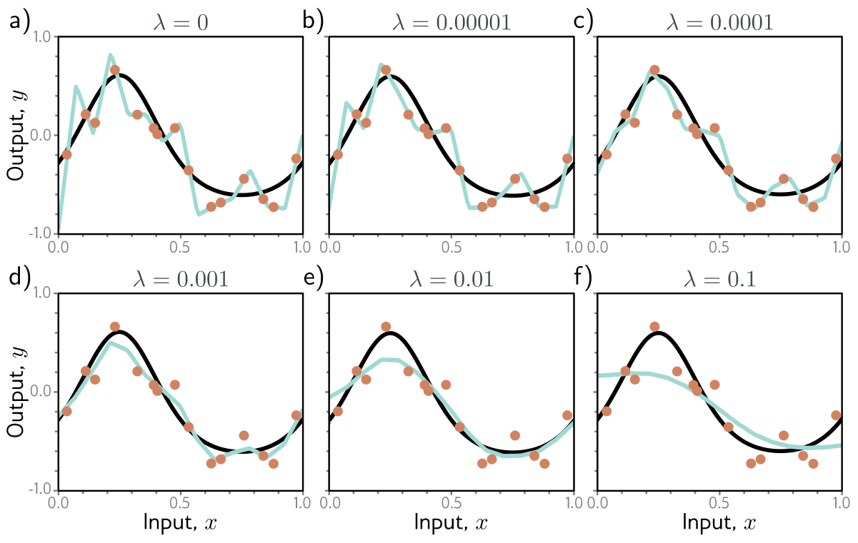
Prince gives two reasons this can improve test performance, and they map onto the two causes of the generalization gap. If the model is overfitting, the penalty forces it to trade “slavish adherence to the data” against smoothness, which in the language of Chapter 8 reduces variance (the model need not pass through every point) at the cost of some bias (it can only describe smooth functions). If the model is over-parameterized, some of its capacity describes regions with no data at all, and there the penalty favors smooth interpolation between the nearest points — a sensible default when nothing else is known.
The simplified model is linear in its parameters, so the L2-regularized fit has a closed form, \((\mathbf{X}^T\mathbf{X} + \lambda\mathbf{P})^{-1}\mathbf{X}^T\mathbf{y}\) with \(\mathbf{P}\) the identity except for a zero in the bias position. That lets us sweep \(\lambda\) over seven orders of magnitude and watch the variance-for-bias trade happen.
best lambda 3.2e-03: error 0.0080; lambda -> 0: 0.0708; lambda = 10: 0.1031Prince, chapter notes, pp. 155–156. The two names are used interchangeably, but they are different algorithms. L2 regularization adds \(\lambda \sum_j
\phi_j^2\) to the loss, so the gradient gains a term \(2\lambda\boldsymbol{\phi}\) (problem 9.2). Weight decay (Hanson and Pratt 1988) instead shrinks the parameters before each gradient step, \[
\boldsymbol{\phi} \longleftarrow (1 - \lambda')\,\boldsymbol{\phi} - \alpha\, \frac{\partial L}{\partial \boldsymbol{\phi}}.
\tag{11}\] For plain SGD the two coincide with \(\lambda = \lambda' / (2\alpha)\) (problem 9.5). For Adam they do not: Adam rescales each coordinate’s gradient — including the \(2\lambda\phi_j\) term — by its own running statistics, so parameters with large gradients are barely regularized. AdamW (Loshchilov and Hutter 2019) applies the decay directly to the parameters as in eq. 11, and torch.optim.AdamW is what the weight_decay argument should mean when you use Adam. In torch.optim.SGD and torch.optim.Adam, weight_decay adds the L2 gradient term instead.
Prince §9.2, p. 141.
Here is the chapter’s most surprising idea. Neither gradient descent nor SGD moves neutrally to the minimum of the loss. Each prefers some solutions to others, and the preference can be written as an extra term in the loss — a regularizer nobody added. This is implicit regularization.
Prince §9.2.1, pp. 141–142; figure on p. 142.
Imagine gradient descent with an infinitesimal step. The parameters then follow the differential equation
\[ \frac{\partial \boldsymbol{\phi}}{\partial t} = -\frac{\partial L}{\partial \boldsymbol{\phi}}, \tag{12}\]
called gradient flow. Real gradient descent approximates it with discrete steps of size \(\alpha\),
\[ \boldsymbol{\phi}_{t+1} = \boldsymbol{\phi}_t - \alpha \frac{\partial L[\boldsymbol{\phi}_t]}{\partial \boldsymbol{\phi}}, \tag{13}\]
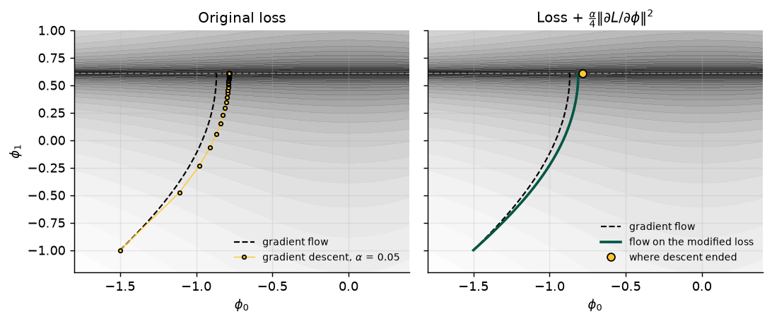
and the discretization makes the path deviate from the continuous one. On a loss with a whole line of global minima (fig. 4a) the two paths end at different points on that line.
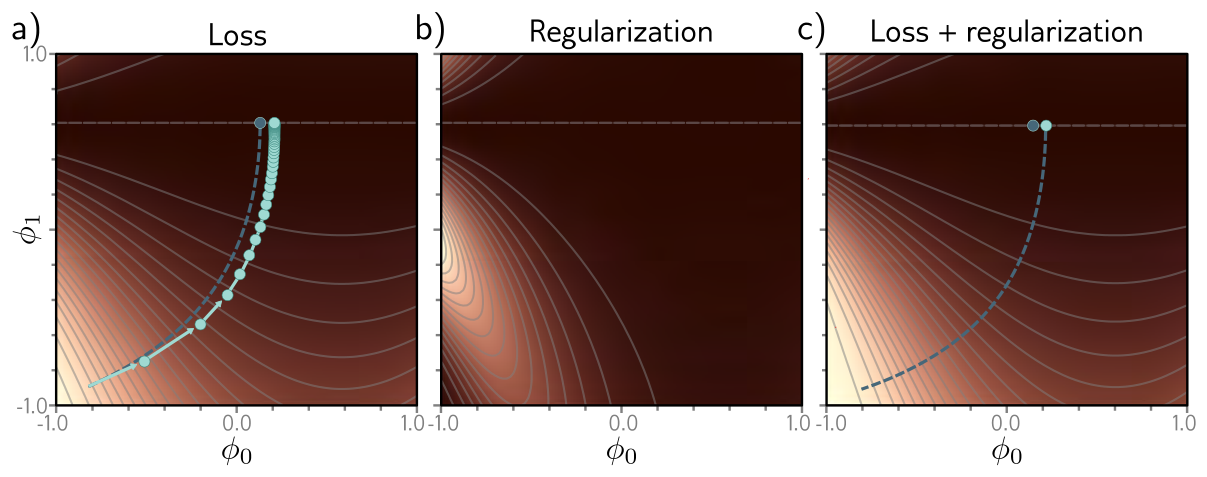
The deviation can be understood by asking a backwards question: on what modified loss \(\tilde{L}\) would the continuous flow arrive where the discrete steps on \(L\) arrived? The chapter notes (pp. 156–157) derive the answer by backward error analysis, keeping terms to second order in \(\alpha\):
\[ \tilde{L}_{\text{GD}}[\boldsymbol{\phi}] = L[\boldsymbol{\phi}] + \frac{\alpha}{4} \left\| \frac{\partial L}{\partial \boldsymbol{\phi}} \right\|^2. \tag{14}\]
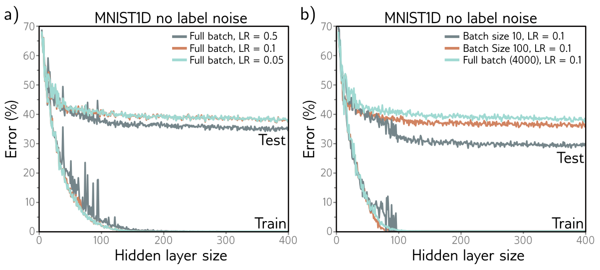
Discrete gradient descent behaves like continuous descent on a loss that penalizes the squared gradient norm. The trajectory is repelled from places where the surface is steep. This does not move the minima — the gradient is zero there anyway — but it changes the loss everywhere else, bends the trajectory, and can send it to a different minimum (fig. 4c). Since the penalty is proportional to \(\alpha\), a larger learning rate regularizes harder, which is one candidate explanation for the observation that full-batch gradient descent generalizes better with larger steps (fig. 7a).
The derivation is first-order in \(\alpha\), so it should match best for small steps. The cell below checks that, on a loss with a line of minima like Prince’s: it runs discrete gradient descent, the continuous flow (approximated by very small steps), and the continuous flow on eq. 14, and reports how much of the discrete path’s deviation the modified loss accounts for.
 alpha  descent ends at  flow ends at  modified flow  deviation explained
  0.02          -0.8386       -0.8670        -0.8419                 89%
  0.05          -0.7857       -0.8670        -0.8112                 69%
   0.1          -0.6352       -0.8670        -0.7722                 41%
0.2 0.0475 -0.8670 -0.7196 16%Prince §9.2.2, p. 144; figure on p. 143.
The same analysis for SGD asks for a modified loss on which the continuous flow lands where the average over the possible random SGD updates lands. The result adds a second term:
\[ \tilde{L}_{\text{SGD}}[\boldsymbol{\phi}] = \tilde{L}_{\text{GD}}[\boldsymbol{\phi}] + \frac{\alpha}{4B} \sum_{b=1}^{B} \left\| \frac{\partial L_b}{\partial \boldsymbol{\phi}} - \frac{\partial L}{\partial \boldsymbol{\phi}} \right\|^2 = L[\boldsymbol{\phi}] + \frac{\alpha}{4} \left\| \frac{\partial L}{\partial \boldsymbol{\phi}} \right\|^2 + \frac{\alpha}{4B} \sum_{b=1}^{B} \left\| \frac{\partial L_b}{\partial \boldsymbol{\phi}} - \frac{\partial L}{\partial \boldsymbol{\phi}} \right\|^2. \tag{15}\]
Here \(L_b\) is the loss of the \(b\)th of the \(B\) batches in an epoch, and both \(L\) and \(L_b\) are now means over their examples:
\[ L = \frac{1}{I} \sum_{i=1}^{I} \ell_i[\mathbf{x}_i, y_i] \qquad\text{and}\qquad L_b = \frac{1}{|\mathcal{B}|} \sum_{i \in \mathcal{B}_b} \ell_i[\mathbf{x}_i, y_i]. \tag{16}\]
The new term is the variance of the batch gradients. SGD implicitly prefers places where all the batches agree about the slope. Like the gradient-descent term, it bends the trajectory (fig. 6) without necessarily moving the global minimum: an over-parameterized model that fits every training point has all batch gradients equal to zero there.
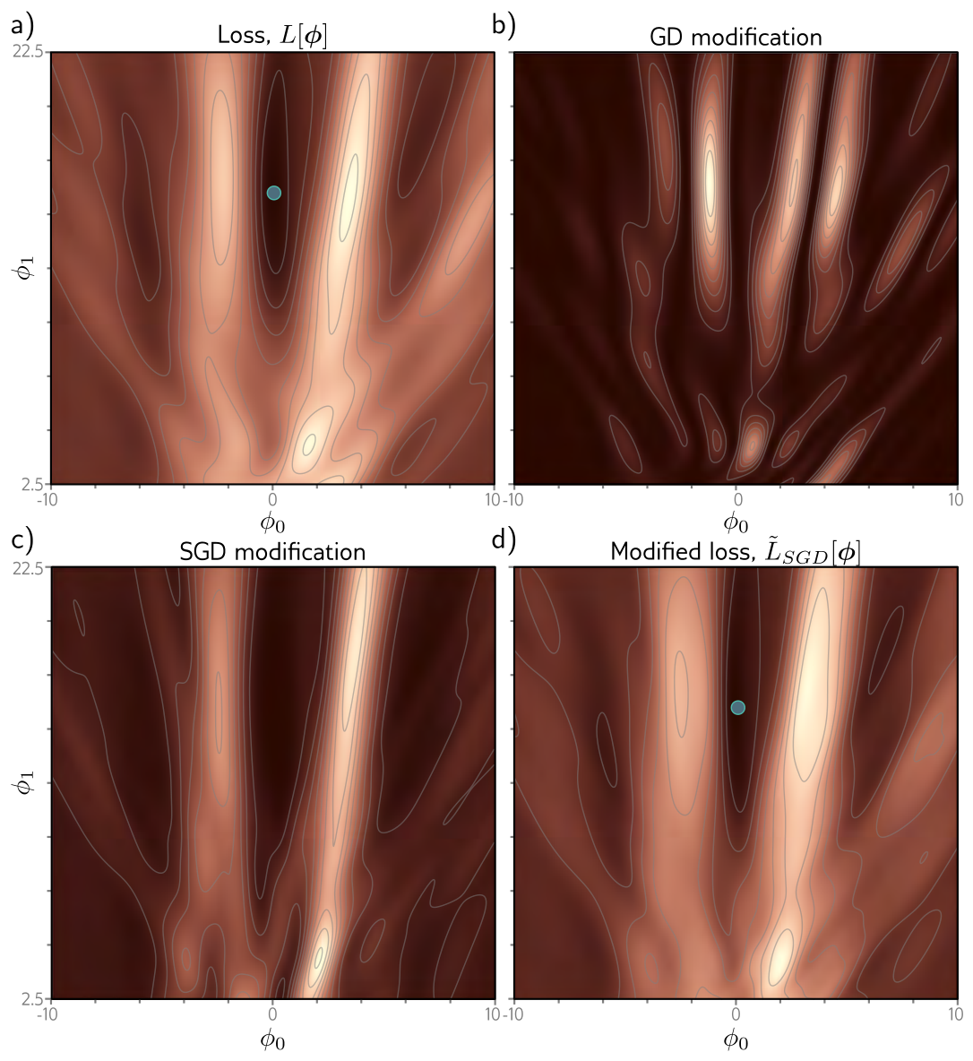
Empirically, SGD generalizes better than gradient descent, and smaller batches generally beat larger ones (fig. 7b). Week 6 offered one explanation, that the noise lets the optimizer reach different parts of the surface. Implicit regularization offers another: SGD is drawn to solutions where all the data fit well — low batch variance — rather than solutions where some examples fit extremely well and others poorly at the same total loss. The former are the ones likely to generalize.
Prince §9.3, p. 144.
Explicit terms and the optimizer’s implicit ones both steer training by changing the loss. The rest of the chapter is a catalog of other devices that improve generalization. Each is simple to state; the interesting part is why it works, and fig. 18 at the end is the map.
Prince §9.3.1, p. 145; figure on p. 146.
Early stopping means halting training before it converges. If the model has already captured the coarse shape of the function but has not yet had time to fit the noise, stopping there reduces overfitting (fig. 8). Two ways to see why. First, the weights start small (Week 7) and simply do not have time to grow large, so early stopping acts like L2 regularization — the chapter notes make this exact for a quadratic loss started from zero, with an effective \(\lambda \approx 1/(\tau\alpha)\) for stopping time \(\tau\) (Goodfellow, Bengio, and Courville 2016). Second, it reduces the effective capacity, moving the model back down the bias–variance curve from the critical region of Chapter 8.
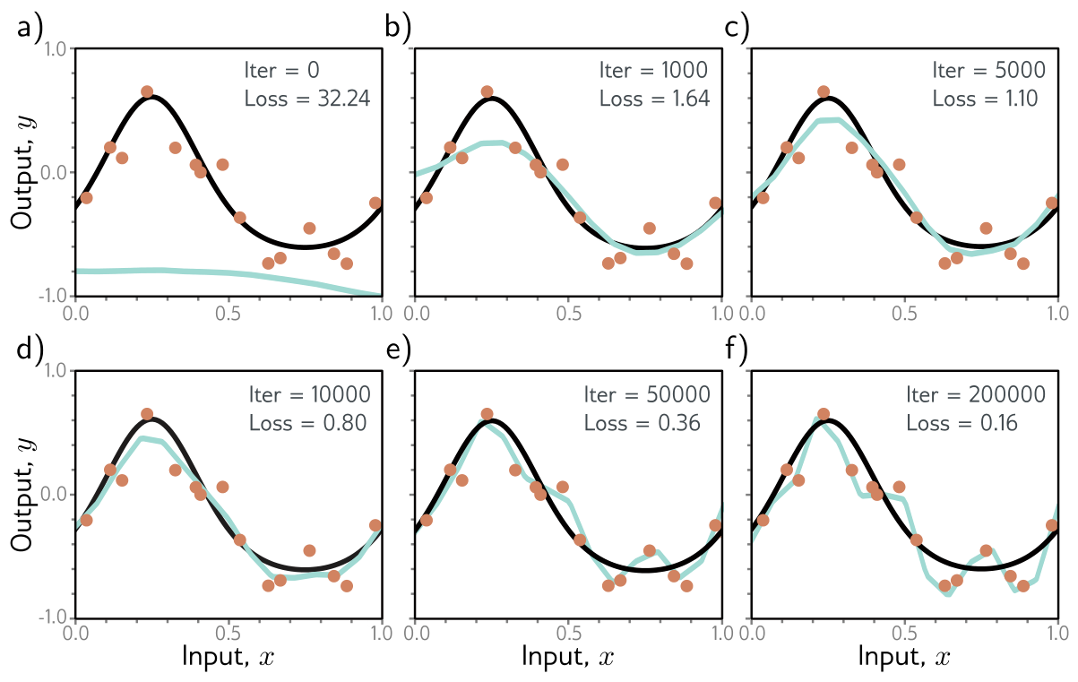
“Reduces the effective complexity” deserves a concrete picture. Training from small initial weights, gradient descent fits the stiff directions of the loss first — the broad features of the function that many data points agree on — and the soft directions, which encode fine wiggles supported by one or two noisy points, only after many more iterations. At any finite stopping time the soft components are still close to their initial value of zero. The model is behaving as if it had fewer free parameters than it has, which is precisely what a small \(\lambda\) in L2 regularization does by shrinking those same components. The figure below puts the two on one axis.
Early stopping has one hyperparameter, the stopping time, chosen on a validation set as usual — but unlike every other hyperparameter it does not require training many models.
One training run yields every candidate stopping time at once; the validation curve is the hyperparameter sweep. In PyTorch this is a few lines around the training loop: best = copy.deepcopy(model.state_dict()) when the validation loss improves, model.load_state_dict(best) at the end.
For our simplified model the whole training trajectory of full-batch gradient descent has a closed form (it is a linear least squares problem, so the flow eq. 12 can be solved exactly through the eigenvectors of \(\mathbf{X}^T\mathbf{X}\)). That makes it possible to plot test error against training time without training anything, and to put it on the same axis as L2 regularization.
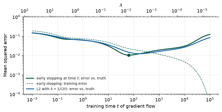
best stopping time t = 63: error 0.0104, training error there 0.0225
trained to convergence: error 0.1226, training error 3.3e-05Prince §9.3.2, pp. 145–147; figure on p. 147.
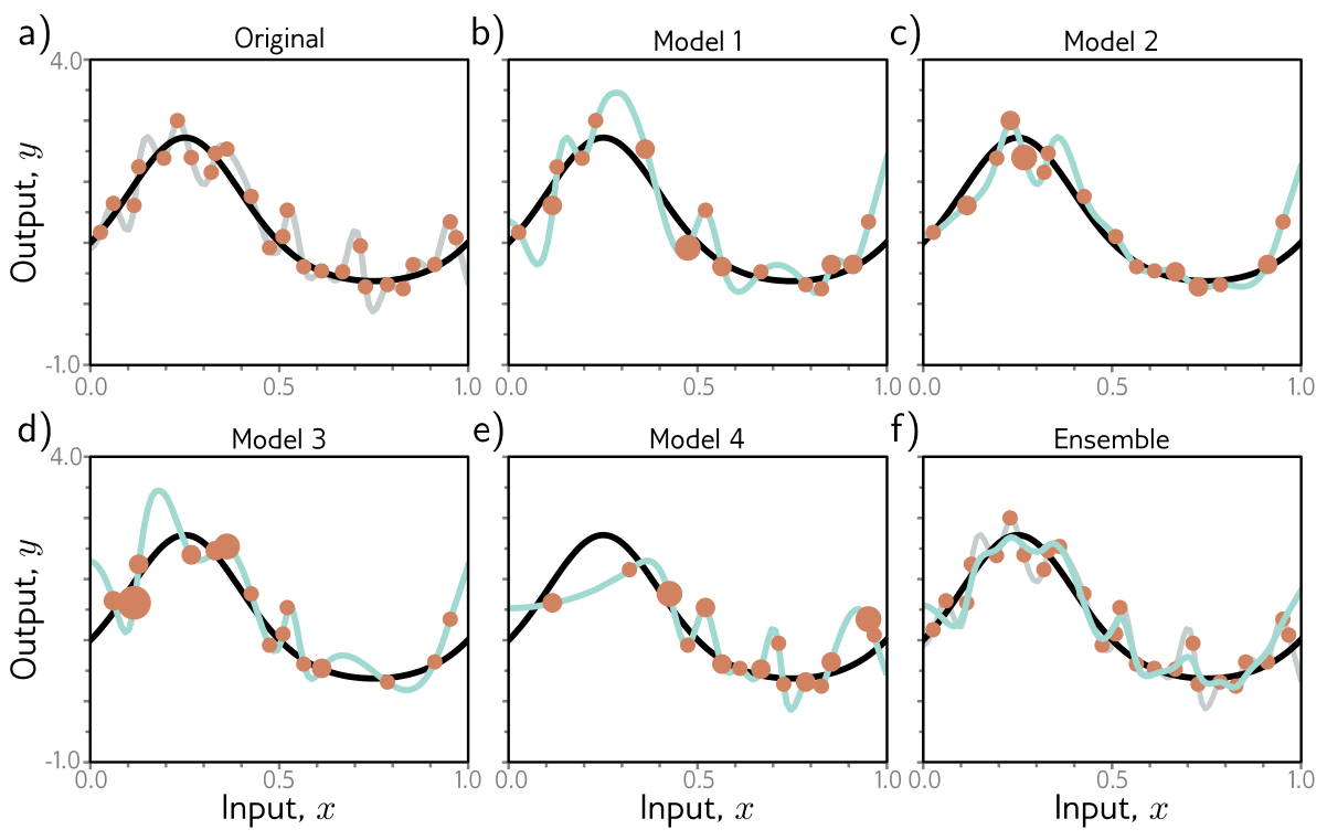
Build several models and average their predictions: an ensemble. This reliably improves test performance — it is the most dependable trick in the chapter — at the cost of training and storing several models and running all of them at inference.
How to combine. For regression, average the outputs. For classification, Prince averages the pre-softmax activations (the logits) rather than the probabilities. Both work; averaging logits amounts to a geometric mean of the models’ probability vectors, which keeps a confident model’s relative preferences intact, whereas averaging probabilities is an arithmetic mean that lets confident and unsure models contribute equally to each class. Taking the median output, or the most frequent predicted class, is a more robust variant: one model that goes badly wrong on an input cannot drag the ensemble with it.
Why it works, and when it does not. The premise is that the models’ errors are independent and cancel. If \(M\) models each have error variance \(\sigma^2\) and the errors of any two are correlated with coefficient \(\rho\), the variance of their average is
\[ \operatorname{Var}\Big[\frac{1}{M}\sum_{m=1}^{M} e_m\Big] = \sigma^2\Big(\rho + \frac{1-\rho}{M}\Big). \tag{17}\]
With independent errors (\(\rho = 0\)) the variance falls like \(1/M\). With correlated errors it never falls below \(\rho\sigma^2\) however many models we add. So an ensemble is only as good as the diversity of its members: ten copies of the same model trained on the same data from the same start are one model. (The bias of each model is untouched by averaging; ensembling is a variance reduction, the third of the four mechanisms.)
Where diversity comes from. The simplest source is different random initializations. This helps most in regions far from the training data, where each model is unconstrained, the models disagree, and their average is more moderate than any one of them. A second source is bagging — bootstrap aggregating (Breiman 1996): draw \(I\) examples with replacement from the \(I\) training points to make a new training set, repeat to make several, and train one model on each (fig. 10). A bootstrap sample contains about 63% of the original points, some of them more than once, and omits the other 37% — the sizes of the orange dots in the figure show the counts. A point left out of one resample is interpolated from its neighbors by that model, so an outlier’s influence is diluted and the average is smoother than any single fit. Other sources of diversity are different hyperparameters, models stored at different times during one training run, or entirely different model families.
error vs. true function, median over 200 training sets:  single model 0.0177   bagged ensemble of 20 0.0132
the ensemble is better on 80% of the training sets
a bootstrap resample of 15 points contains on average 65% distinct points (the limit is 1 - 1/e = 63%)Prince §9.3.3, pp. 147–149; figures on pp. 148–149.
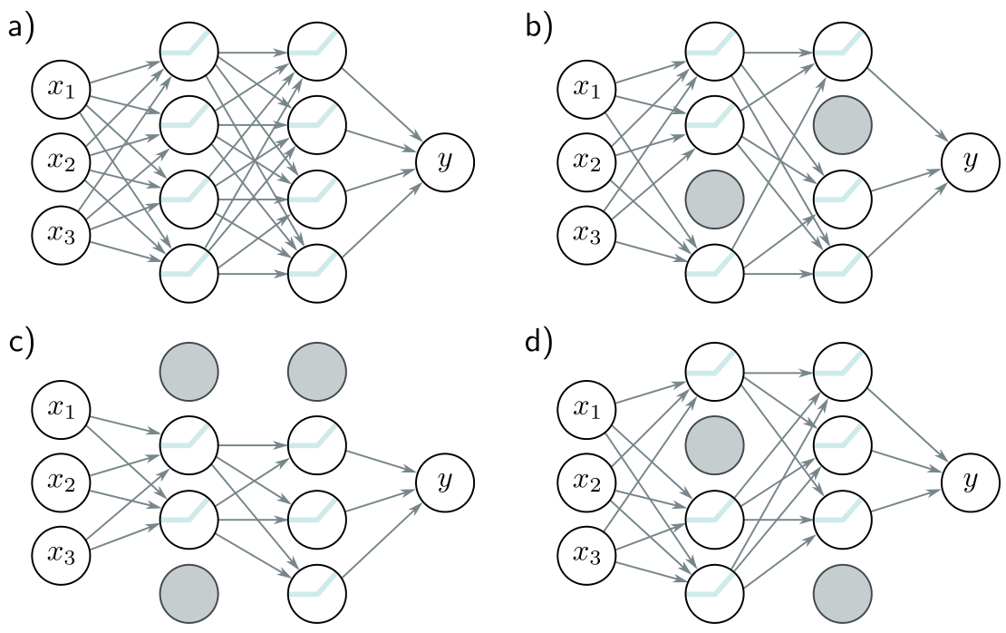
Dropout randomly clamps a subset of hidden units — typically half — to zero at every SGD iteration (fig. 11). Clamping a unit to zero is the same as temporarily removing it: its incoming weights receive no gradient and its outgoing weights contribute nothing, so each step trains a slightly different, thinner network, and the next step a different one again.
Two consequences follow. First, the network cannot rely on any particular unit, because that unit may be absent when the loss is computed. A feature that is only useful in combination with three specific other units — a “co-adaptation” — is fragile under dropout, so the training pressure favours units that are individually useful. Second, the weights are pushed smaller: when a unit disappears, the function changes by the size of that unit’s contribution, and the loss penalizes large swings, so the network learns to spread its function over many small contributions rather than a few large ones. That is the same smoothness L2 regularization buys, obtained by a different route.
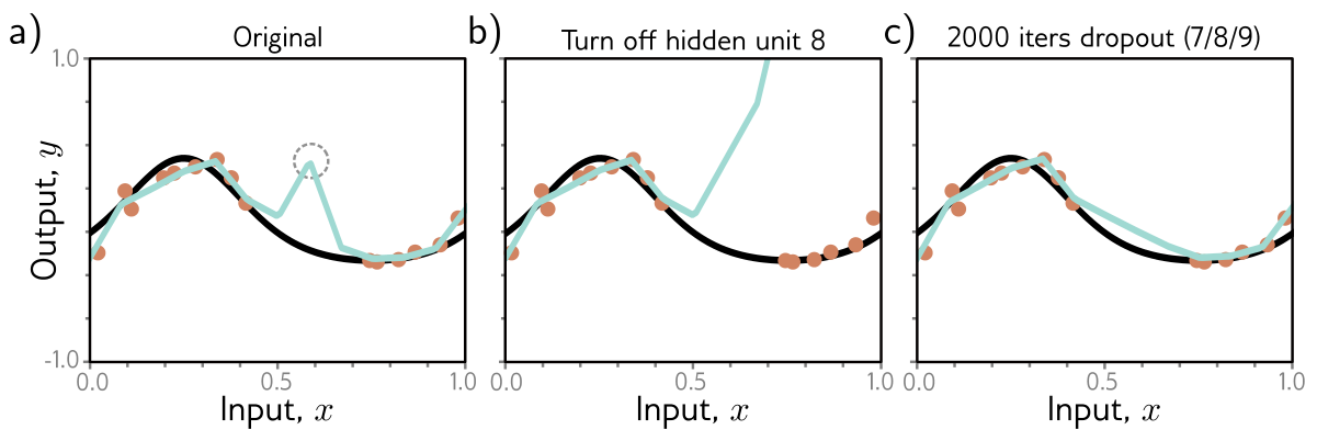
Prince’s mechanism for why this generalizes is worth following closely (fig. 12). Suppose three hidden units become active one after another along the input axis. The first raises the slope sharply, the second lowers it, the third cancels the decrease and returns the curve to its path. Together they make a kink between two data points that contributes nothing to the training loss — the model already fits the data as well as it can — so gradient descent will never remove it, yet it is unlikely to reflect the truth. Now drop the middle unit. Without its decrease, everything to the right of that joint swings upward and the loss jumps; the next gradient step compensates, and over many iterations these conspiracies between units are dismantled. Dropout removes large, unnecessary changes between training points even though they cost nothing.
At test time there are two options.
Weight scaling inference rule. Run the full network with every unit on. But the next layer was trained on inputs where each unit was present only a fraction \(1 - p\) of the time: during training the expected contribution of unit \(j\) to a downstream pre-activation was \((1 - p)\,\omega_j h_j\). With every unit present the contribution is \(\omega_j h_j\), larger by \(1/(1 - p)\), and the pre-activations would be systematically too big. So multiply the weights by \(1 - p\) at inference (with \(p = 0.5\), halve them) to restore the expectation the network was trained under. This is a single deterministic pass and costs nothing.
Monte Carlo dropout (Gal and Ghahramani 2016). Alternatively, keep dropout on at test time, run the network several times with different random subsets of units clamped to zero, and average the results. Every random thinning is a different model, so this is an ensemble — but one whose members share a single set of weights and so never had to be trained or stored separately. The spread of the passes is a rough measure of the model’s uncertainty, which the single deterministic pass cannot give.
nn.Dropout(p) zeroes each input with probability p and multiplies the survivors by \(1/(1-p)\) during training (the inverted form of the scaling rule, so that no rescaling is needed later). model.eval() turns it off for inference; model.train() turns it back on, which is how Monte Carlo dropout is done. Forgetting model.eval() before testing is a classic bug.
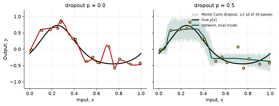
eval() mode, the fit is smoother, misses the noisiest points, and its error is 0.013, almost three times smaller. The shaded band spans \(\pm 2\) standard deviations of 30 Monte Carlo dropout passes of the same network; it is widest where the data are sparsest, which is the uncertainty estimate that comes free with dropout.
p = 0.0: error vs. truth 0.0360 (eval mode), 0.0360 (mean of 30 Monte Carlo passes)
p = 0.5: error vs. truth 0.0140 (eval mode), 0.0143 (mean of 30 Monte Carlo passes)Prince §9.3.4, pp. 149–150; figure on p. 150.
Dropout is multiplicative Bernoulli noise on the activations. Once you see it that way, noise can be applied anywhere in the network during training, and in each place it buys a different kind of robustness.
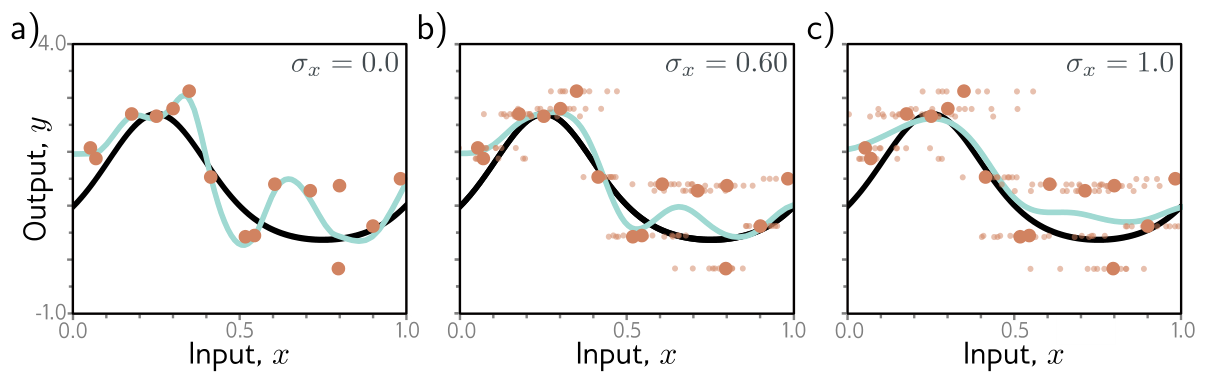
Noise on the inputs smooths the learned function (fig. 14). At each SGD step, each input \(\mathbf{x}_i\) in the batch is replaced by \(\mathbf{x}_i + \boldsymbol{\epsilon}_i\) with fresh Gaussian noise of variance \(\sigma^2_x\). The model can no longer pin a prediction to one exact input; it has to predict about the same thing across a small neighbourhood, which is what “smooth” means. For regression this is equivalent to adding a penalty on the derivatives of the output with respect to the input (Bishop 1995), and for a straight line the equivalence is exact.
For \(y = \phi_0 + \phi_1 x\) with the least squares loss, add noise \(\epsilon_i \sim \mathrm{Norm}[0, \sigma^2_x]\) to each input. One term of the loss is \[ \big(\phi_0 + \phi_1(x_i + \epsilon_i) - y_i\big)^2 = \big(\phi_0 + \phi_1 x_i - y_i\big)^2 + 2\phi_1\epsilon_i\big(\phi_0 + \phi_1 x_i - y_i\big) + \phi_1^2\epsilon_i^2. \] Taking the expectation over the noise kills the middle term (\(\mathbb{E}[\epsilon_i] = 0\)) and turns the last into \(\phi_1^2\sigma^2_x\). Summed over the \(I\) examples, \[ \mathbb{E}_{\epsilon}\big[L_{\text{noisy}}[\boldsymbol{\phi}]\big] = L[\boldsymbol{\phi}] + I\sigma^2_x\,\phi_1^2, \tag{18}\] the original loss plus an L2 penalty on the slope \(\phi_1 = \partial y / \partial x\) — the derivative of the output with respect to the input — with \(\lambda = I\sigma^2_x\). The intercept is not penalized, because shifting the line up or down does not change how sensitive it is to the input. The expected gradient update is therefore the usual one plus \(2 I \sigma^2_x \phi_1\) on the slope alone. For a nonlinear network the same calculation holds locally: input noise penalizes \(\|\partial \mathrm{f} / \partial \mathbf{x}\|^2\) averaged over the training inputs.
expected loss with input noise (Monte Carlo):   6.3178
L + I sigma_x^2 phi_1^2, equation (input noise): 6.3158
The extreme version is adversarial training, in which the optimizer does not sample the perturbation at random but actively searches for the small \(\boldsymbol{\epsilon}_i\) that most increases the loss — the worst-case noise — and trains against that.
Noise on the weights asks the network to predict sensibly even when its parameters are slightly wrong. Picture two minima of the loss with the same depth: one at the bottom of a narrow, sharp valley, one in the middle of a wide, flat basin. Perturb the parameters by a small random amount and the loss at the sharp minimum jumps, while the loss at the flat one barely moves. Training on the expected loss under weight noise — to second order, \(L[\boldsymbol{\phi}] + \tfrac{1}{2}\sigma^2_\phi\,\mathrm{tr}[\mathbf{H}]\), a penalty on the curvature — therefore steers toward wide, flat minima, where the individual weights do not matter much. Such solutions are robust to the estimation error in every weight, which is the fourth of the four mechanisms.
Noise on the labels. The multiclass cross-entropy wants to predict the correct class with certainty, which drives the pre-softmax activations toward \(\pm\infty\) (Week 8’s overconfidence). Suppose instead that a fraction \(\rho\) of the labels are wrong and belong, with equal probability, to one of the other classes. One could flip labels at random each iteration; the same effect comes from changing the target of the cross-entropy to a distribution with \(1 - \rho\) on the true class and \(\rho/(K-1)\) on each of the others. This is label smoothing (Szegedy et al. 2016), and it helps across many tasks, although the mechanism is not fully understood; it does improve the calibration of the predicted probabilities (Müller, Kornblith, and Hinton 2019).
Writing the smoothed loss out (problem 9.4) shows what it does. With \(K\) classes, predicted probabilities \(p_k\) from the softmax, true class \(y\), and a target that puts \(1 - \rho\) on \(y\) and \(\rho / (K - 1)\) on each other class, the cross-entropy between target and prediction is
\[ \ell = -(1 - \rho)\log p_y - \frac{\rho}{K - 1}\sum_{k \neq y} \log p_k = (1 - \rho)\,\underbrace{\big[-\log p_y\big]}_{\text{usual loss}} + \rho\,\underbrace{\Big[-\frac{1}{K-1}\sum_{k \neq y}\log p_k\Big]}_{\text{keeps every class alive}}. \tag{19}\]
The first term is the ordinary cross-entropy of Chapter 5, down-weighted by \(1 - \rho\). The second term is new: it grows without bound if any wrong class’s probability is driven to zero, so the network is penalized for being certain. The smoothed target cannot be matched by an infinitely confident prediction, and the logits stop growing — and we can say exactly where.
K = 10 classes, rho = 0.1: the smoothed cross-entropy is minimized at a logit gap of 4.394
closed form log[(1 - rho)(K - 1) / rho] = 4.394
minimum loss 0.5448 = entropy of the target 0.5448  (not zero: the target is not one-hot)
with rho = 0 the loss keeps falling as the gap grows: gap 15 gives 2.75e-06, gap 30 gives 8.42e-13
With ten classes and \(\rho = 0.1\), the loss is minimized when the correct logit exceeds the others by \(\log 81 \approx 4.4\) and no further — a probability of 0.9 on the true class, exactly the target. Problem 9.4 asks for the general loss.
Prince §9.3.5, pp. 150–151; figure on p. 151.
Maximum likelihood is overconfident by construction: it picks the single most likely parameter vector and predicts as if it were certainly right, when many other parameter vectors are nearly as compatible with the data. The Bayesian approach treats the parameters as unknown and computes a whole distribution over them given the training data, by Bayes’ rule:
\[ Pr(\boldsymbol{\phi} \mid \{\mathbf{x}_i, y_i\}) = \frac{\prod_{i=1}^{I} Pr(y_i \mid \mathbf{x}_i, \boldsymbol{\phi})\, Pr(\boldsymbol{\phi})}{\int \prod_{i=1}^{I} Pr(y_i \mid \mathbf{x}_i, \boldsymbol{\phi})\, Pr(\boldsymbol{\phi})\, d\boldsymbol{\phi}}. \tag{20}\]
The numerator is the MAP objective of eq. 4; the denominator normalizes it into a probability. Prediction for a new input then integrates over every parameter setting, weighting each by its posterior probability:
\[ Pr(y \mid \mathbf{x}, \{\mathbf{x}_i, y_i\}) = \int Pr(y \mid \mathbf{x}, \boldsymbol{\phi})\, Pr(\boldsymbol{\phi} \mid \{\mathbf{x}_i, y_i\})\, d\boldsymbol{\phi}. \tag{21}\]
This is an infinite ensemble, weighted by prior plausibility and agreement with the data, and it returns a predictive distribution — a mean and an uncertainty — rather than a point (fig. 15). The prior variance plays the role of \(\lambda\): a tight prior gives smoother sampled functions.
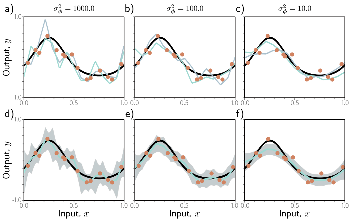
For the simplified network the posterior is a Gaussian and eq. 21 can be computed exactly. For a deep network there is no practical way to represent a distribution over millions of parameters or to integrate over it; every working method approximates, by a simpler distribution (variational Bayes) or by samples (MCMC), and adds considerable complexity. Monte Carlo dropout can be read as a cheap approximation of this kind.
Prince §9.3.6, pp. 151–152; figure on p. 153.
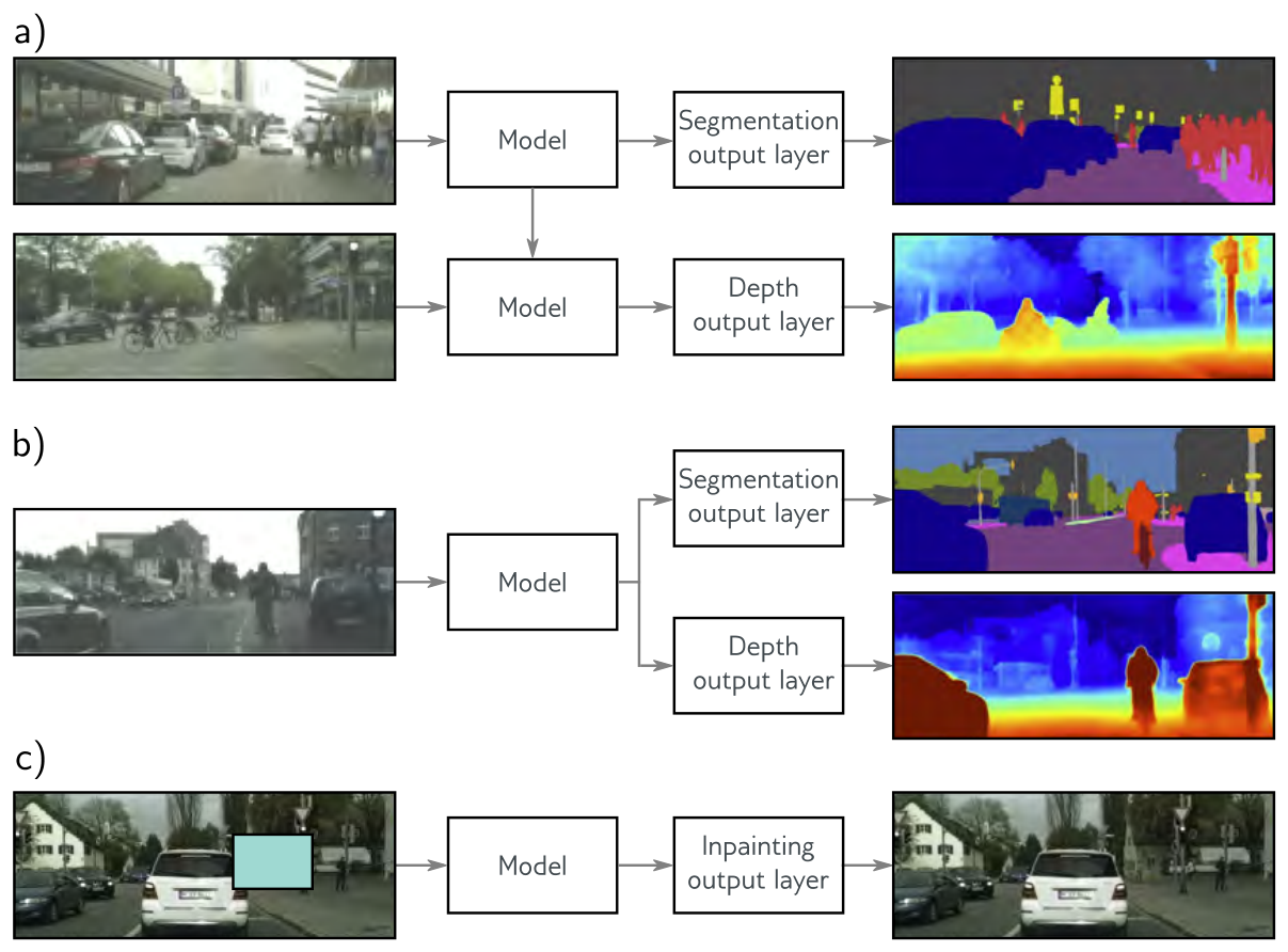
When labeled data for the task are scarce, use someone else’s data. In transfer learning (fig. 16a) the network is first pre-trained on a related secondary task for which data are plentiful — a million labeled photographs, say, or every image on the web with its caption. Then the last layer, which produced the secondary task’s outputs, is removed, and one or more new layers that produce the outputs we actually want are added in its place. From here there are two choices:
The premise is that the secondary task teaches a good internal representation of the data: the early layers of an image network learn edges, textures, and parts that are useful for almost any image task, and only the last layers are specific to the labels they were trained on. Equivalently, pre-training initializes most of the parameters in a part of parameter space from which a good solution is reachable — Chapter 7’s view of initialization, extended from “keep the variances level” to “start from a network that already sees.” The cell below shows the mechanics on a standard image network.
ResNet-18: 11,689,512 parameters; its last layer is Linear(in_features=512, out_features=1000, bias=True)
frozen backbone + new head: 2,052 trainable parameters (0.02% of the model)
also fine-tuning the last residual block: 8,395,780 trainable parameters
With the backbone frozen, a four-class classifier has two thousand free parameters — a model a few hundred labeled images can constrain — sitting on top of eleven million that were constrained by someone else’s million images. That is the sense in which transfer learning “increases the data.”
Multi-task learning (fig. 16b) trains one network on several tasks at once — segment the scene, estimate depth, caption the image — with a shared trunk and one output head per task, and a loss that is a weighted sum of the tasks’ losses. The grounds are that all of the tasks require understanding the image, so each task’s labels constrain the shared representation and each may improve the others. Where transfer learning borrows a dataset, multi-task learning borrows labels for the same inputs.
Prince §9.3.7, p. 152.
Transfer learning needs a secondary task with labels. Self-supervised learning manufactures them from unlabeled data, and there are two families. In generative self-supervision part of each example is masked and the task is to predict it: inpaint a missing patch of an image (fig. 16c), or predict masked words in a text corpus — which is how the language models of Chapter 12 are pre-trained (Devlin et al. 2019). In contrastive self-supervision the task is to tell whether two examples are related: two transformed views of the same image versus views of different images (Chen et al. 2020), or two sentences that did or did not follow one another in a document.
The point in both families is that the labels are free: they are manufactured from the data itself, so the secondary task can use every unlabeled example we have. The network trained on it is then transferred exactly as above — head removed, new head added, frozen or fine-tuned. For an industrial sensor stream the generative version is natural: mask one channel, or one time window, and train the network to predict it from the rest; what it learns about how the channels relate is then a starting point for the fault-detection task with its few hundred labels.
Prince §9.3.8, pp. 152–154; figure on p. 154.
Transfer learning borrows a dataset; multi-task learning borrows labels; data augmentation expands the dataset we have. Many inputs can be transformed in ways that leave the label unchanged: rotate, flip, crop, blur, or recolor an image of a bird and it is still a bird (fig. 17); substitute synonyms in a sentence or translate it to another language and back; amplify or attenuate frequency bands of an audio clip. The augmented examples teach the model to be indifferent to these irrelevant transformations. AlexNet (Krizhevsky, Sutskever, and Hinton 2012) multiplied its training set by 2,048 this way.
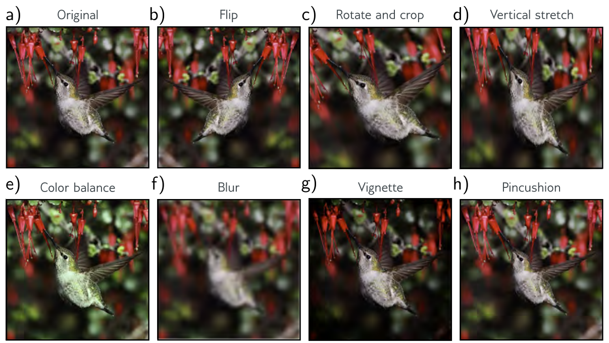
In a manufacturing image task the right augmentations depend on the physics. A part on a conveyor may appear at any rotation, so rotations are safe; but a horizontal flip of a part with a chirality — a left-hand versus right-hand bracket — changes its class. A brightness shift mimics a change of lighting; a blur may erase exactly the fine scratch the inspector is looking for. For sensor time series, time-shifting a window is usually safe while time-reversing it rarely is. Write down what each transformation assumes before you use it.
Prince §9.4, pp. 154–155; figure on p. 155.
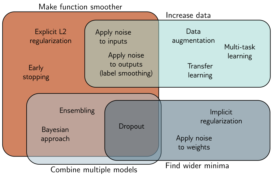
Prince’s summary diagram places every method in this chapter in one or more of four regions. The reasons they work are not as varied as the methods.
| Mechanism | What it changes | Methods |
|---|---|---|
| Make the function smoother | Reduces variance; favors smooth interpolation where there is no data | L2 regularization, early stopping, input noise, label smoothing |
| Increase the data | Constrains the function in more of the input space | Data augmentation, transfer learning, multi-task learning |
| Combine multiple models | Averages out errors that differ between fits | Ensembling, bagging, Bayesian inference, dropout |
| Find wider minima | Makes the solution robust to errors in the parameters | Weight noise, dropout, implicit regularization of SGD |
One more lever sits outside this chapter: choose an architecture that suits the task. In image segmentation, sharing parameters across positions means the network need not learn what a tree looks like separately at every pixel. The cell below says how large that saving is.
fully connected layer, every pixel to 1,000 units:  150,528,000 weights
3x3 convolution with 64 channels, shared everywhere:        1,792 parameters
ratio: 84,000 to 1
A convolution is a fully connected layer with two constraints built in: each unit looks only at a small patch, and every position uses the same weights. Those constraints are a prior — “what matters is local, and it matters the same way everywhere in the image” — enforced by the architecture rather than by a penalty, and they remove tens of thousands of parameters per unit that would otherwise have to be constrained by data. Chapters 10–13 are about such architectural choices, and the next of them, convolution, is the biggest regularizer in computer vision.
Start from a pre-trained model if one exists for your modality, and fine-tune. Use augmentations that the physics permits. Train with SGD or AdamW, weight decay on, with a validation set monitored for early stopping. Add dropout before the output layer if the training–validation gap is still large. If you can afford it, ensemble a few seeds; if you cannot, use Monte Carlo dropout to get an uncertainty estimate. Label-smooth a classifier whose probabilities will be used (thresholded, ranked) rather than just argmax-ed. Every one of these is a hyperparameter chosen on validation data, never on the test set.
Prince §9.4, p. 154.
Explicit regularization adds a term to the loss that moves its minimum; read as a prior over the parameters, L2 regularization is a zero-mean normal prior and makes the function smoother, trading variance for bias. Gradient descent with a finite step does not descend the loss we wrote: to first order it descends the loss plus \(\frac{\alpha}{4}\) times the squared gradient norm, and SGD adds a penalty on the variance of the batch gradients — implicit regularization that favors flat regions where all the data agree, and that grows with the learning rate and shrinks with the batch size. Beyond these, a family of heuristics improves generalization: early stopping (which mimics L2), ensembling and bagging, dropout (which dismantles conspiracies between units and is an ensemble in disguise), noise on inputs, weights, or labels, the Bayesian approach (an infinite ensemble), transfer, multi-task and self-supervised learning, and data augmentation. All of them act through four mechanisms: a smoother function, more data, combined models, or a wider minimum.
Next: Chapter 10 changes the architecture. Convolutional networks build translation invariance into the model itself, so that a pattern learned at one position in an image is recognized everywhere — the most consequential regularizer in computer vision, and the first architecture designed around the structure of the data.
1. (UDL 9.1) The prior over the parameters is \(Pr(\boldsymbol{\phi}) = \prod_{j=1}^{J} \mathrm{Norm}_{\phi_j}[0, \sigma^2_\phi]\). Show that maximizing \(\prod_i Pr(y_i \mid \mathbf{x}_i, \boldsymbol{\phi})\, Pr(\boldsymbol{\phi})\) gives a loss equivalent to L2 regularization, and express \(\lambda\) in terms of \(\sigma^2_\phi\). Which way does \(\lambda\) move when the prior gets tighter?
2. (UDL 9.2 and 9.5) How does the gradient of the loss change when the L2 term of eq. 8 is added? Then show that the weight decay update eq. 11 on the original loss equals a plain gradient step on \(\tilde{L}[\boldsymbol{\phi}] = L[\boldsymbol{\phi}] + \frac{\lambda'}{2\alpha} \sum_k \phi_k^2\). Why does this equivalence fail for Adam?
3. (UDL 9.3*) For linear regression \(y = \phi_0 + \phi_1 x\) with a least squares loss, Gaussian noise of variance \(\sigma^2_x\) is added to each input at every training iteration. Compute the expected gradient update and identify the regularization term it implies.
4. (UDL 9.4*) Derive the loss for multiclass classification with label smoothing, when the target puts 0.9 on the correct class and spreads 0.1 over the other \(D_o - 1\) classes. Then use the label-smoothing cell to find the optimal logit gap for \(D_o = 3\) and compare with the closed form.
5. (UDL 9.6) For \(\boldsymbol{\phi} = [\phi_0, \phi_1]^T\), sketch the \(L_0\), \(L_{1/2}\), and \(L_1\) regularization terms \(\sum_d |\phi_d|^P\) in the style of fig. 1b. Using the chapter notes (p. 156), explain why \(L_1\) produces sparser solutions than \(L_2\) and why \(L_0\) is hard to optimize.
6. Equation eq. 14 says gradient descent penalizes the squared gradient norm, with a coefficient proportional to \(\alpha\). (a) Why does this not change the location of any minimum? (b) Using fig. 7a, explain the sense in which a large learning rate “regularizes”. (c) The table under fig. 5 shows the modified loss explaining 90% of the deviation at \(\alpha = 0.02\) but only a small fraction at \(\alpha = 0.2\). Why?
7. Dropout, bagging, and Monte Carlo dropout all appear under “combine multiple models” in fig. 18. For each, say what the individual models are, how many of them are trained, how many are stored, and how the combination is formed at inference. Which one also appears under “find wider minima”, and why?
8. Choosing a strategy. A plant has 600 labeled thermal images of welds (80 defective) and wants a classifier. (a) Rank, with reasons, the first three regularization techniques you would try. (b) Which augmentations are safe for thermal weld images and which are not? (c) The team reports 99% training accuracy and 84% validation accuracy, and asks whether to add more layers or remove some. What do you answer, and which of the four mechanisms are you invoking?
9. Computational. In the fig-l2-sweep cell, the bias is excluded from the penalty. Include it, and compare the sweep. Then replace the L2 penalty by an L1 penalty (you will need an iterative solver; scipy.optimize.minimize on the regularized loss is enough) and count how many of the 14 weights are exactly zero (below \(10^{-6}\)) at the best \(\lambda\).
10. Computational. Extend the fig-dropout cell: (a) sweep \(p \in \{0.1,
0.3, 0.5, 0.7\}\) and plot error against \(p\); (b) implement the weight-scaling rule by hand — train with nn.Dropout replaced by your own Bernoulli mask with no rescaling, then multiply the weights of the following layer by \(1 - p\) at inference — and verify it agrees with eval() mode on the PyTorch version.
11. Computational. Early stopping in practice: return to the Week 8 fig-overconfident experiment, hold out 100 of the 400 training examples as a validation set, and stop at the step with the lowest validation loss. Report test error and test loss at that step and at the end of training. Then add weight_decay=1e-3 to the optimizer and nn.Dropout(0.5) after each hidden layer and repeat. Which of the three interventions most reduced the test loss, and which the test error?
Every part of this page, mapped to Prince, Understanding Deep Learning (MIT Press, 2024) (Prince 2024). Page numbers are those of the printed book.
| This page | Prince section | Pages | Figures used |
|---|---|---|---|
| Why Another Chapter on the Generalization Gap | Ch. 9 opening | 138 | — |
| Explicit Regularization | §9.1 | 138–139 | 9.1 (p. 139) |
| — Probabilistic interpretation | §9.1.1 | 139–140 | — |
| — L2 regularization | §9.1.2; notes | 140–141, 155–156 | 9.2 (p. 141) |
| Implicit Regularization | §9.2 | 141 | — |
| — in gradient descent | §9.2.1; notes | 141–142, 156–157 | 9.3 (p. 142) |
| — in stochastic gradient descent | §9.2.2 | 144 | 9.4 (p. 143), 9.5 (p. 145) |
| Heuristics to Improve Performance | §9.3 | 144 | — |
| — Early stopping | §9.3.1; notes | 145, 157 | 9.6 (p. 146) |
| — Ensembling | §9.3.2; notes | 145–147, 158 | 9.7 (p. 147) |
| — Dropout | §9.3.3; notes | 147–149, 158 | 9.8 (p. 148), 9.9 (p. 149) |
| — Applying noise | §9.3.4; notes | 149–150, 158 | 9.10 (p. 150) |
| — Bayesian inference | §9.3.5; notes | 150–151, 159 | 9.11 (p. 151) |
| — Transfer learning and multi-task learning | §9.3.6; notes | 151–152, 159 | 9.12 (p. 153) |
| — Self-supervised learning | §9.3.7; notes | 152, 159 | — |
| — Augmentation | §9.3.8; notes | 152–154, 159–160 | 9.13 (p. 154) |
| Four Mechanisms | §9.4 | 154–155 | 9.14 (p. 155) |
| Summary | §9.4 | 154 | — |
| Exercises 1–5 | Problems 9.1–9.6 | 160 | — |
Equations on this page correspond to Prince as follows: eq. 1 is his (9.1), eq. 2 is (9.2), eq. 3 is (9.3), eq. 4 is (9.4), eq. 8 is (9.5), eq. 12 is (9.6), eq. 13 is (9.7), eq. 14 is (9.8), eq. 15 is (9.9), eq. 16 is (9.10), eq. 20 is (9.11), eq. 21 is (9.12), and eq. 11 is (9.13). Equations eq. 5, eq. 6 and eq. 7 work problem 9.1, eq. 9 and eq. 10 work problems 9.2 and 9.5, eq. 18 works problem 9.3, eq. 19 works problem 9.4, and eq. 17 is ours.
Figures 9.1–9.14 are reproduced unaltered from Prince, Understanding Deep Learning (MIT Press, 2024), which is distributed under a Creative Commons CC-BY-NC-ND license, and are used here for non-commercial classroom instruction. Original sources credited within the figures: the images in figure 9.12 are from Cordts et al. (2016), the Cityscapes dataset, and figure 9.13 is adapted from Wu et al. (2015a). All other figures on this page are generated by the code in this week’s notebook.