parameter      backprop  finite diff.     autograd
beta_0       0.07743275    0.07743275   0.07743275
omega_0      0.17809533    0.17809533   0.17809533
beta_1      -0.11131057   -0.11131057  -0.11131057
omega_1     -0.01239568   -0.01239568  -0.01239568
beta_2       0.23164291    0.23164291   0.23164291
omega_2      0.18551762    0.18551762   0.18551762
beta_3       0.92963762    0.92963762   0.92963762
omega_3      0.89329789    0.89329789   0.89329789

d l / d omega_0 from the brute-force equation (7.7): 0.17809533Gradients and Initialization
Week 7 · Sessions 13–14 · October 6 & 8, 2026
training
Two problems specific to neural networks: computing the gradient of a loss with respect to millions of parameters efficiently, which is backpropagation, and choosing initial parameters so that neither the activations nor the gradients vanish or explode on their way through the network.
How to read the references in these notes
Every section below opens with the section number and page range it covers in Prince, Understanding Deep Learning (MIT Press, 2024). Page numbers are those of the printed book. Figures taken from the textbook are captioned with their original figure number and page; figures generated by the code behind this page are ours. A complete cross-reference table appears in Section 11.
1 Learning Objectives
By the end of this week you should be able to:
- Name the two problems this chapter solves and explain why each is specific to neural networks rather than to optimization in general.
- State the two observations behind backpropagation — weight gradients scale with the source activation, and downstream derivatives can be computed once and reused — and connect each to the forward and backward pass.
- Carry out the forward pass and both backward passes by hand for the scalar toy model of §7.3, and check the result against finite differences.
- Write the backpropagation algorithm for a deep ReLU network in matrix form, give the shape of every term, and implement it with nothing but matrix products and an indicator mask.
- Explain why backpropagation is cheap in arithmetic but expensive in memory, and estimate both for a given network.
- Describe what algorithmic differentiation frameworks do, how a batch becomes a tensor, and why any acyclic computational graph can be differentiated the same way.
- Show from the variance recursion why poorly scaled weights make activations and gradients vanish or explode, and derive He initialization, its backward-pass counterpart, and the compromise between them.
- Recognize the symptoms of a bad initialization in a network that will not train, and know which initialization PyTorch uses unless you tell it otherwise.
The code lives in a notebook
This page shows the figures and results; the Python behind them is not printed here. All of it — every cell, in the order the note uses it — is in a notebook you can open in the browser with nothing to install:
- ▶ Open the Week 7 notebook in Google Colab — all of this page’s code, in order.
- ▶ Open A3 in Google Colab — the midterm review assignment, Chapters 1–7 in code; nothing to install.
- ▶ UDL notebook 7.1 — Backpropagation in toy model — the forward and backward passes of §7.3, one line at a time.
- ▶ UDL notebook 7.2 — Backpropagation — eq. 21–eq. 23 for a deep ReLU network.
- ▶ UDL notebook 7.3 — Initialization — the experiment of fig. 8.
Colab gives you a Python environment with NumPy, matplotlib, and PyTorch already installed. In Colab, run a cell with Shift+Enter. If you prefer to work locally, pip install -r requirements.txt from the course repository gives you the same environment.
2 Two Problems Specific to Neural Networks
Prince, Chapter 7 opening, p. 96.
Week 6 treated optimization in general. Choose initial parameters at random, then make a series of small changes that decrease the loss on average, each change based on the gradient of the loss with respect to the parameters at the current position. Nothing in that loop cared whether the model was a line, a Gabor function, or a network.
Two things about it become hard — and specific — once the model is a deep network, and they are the two halves of this chapter.
- Computing the gradient efficiently. The largest models at the time Prince wrote have on the order of \(10^{12}\) parameters, and the gradient must be computed for every parameter at every iteration. A method whose cost grows with the number of parameters times the cost of evaluating the network is hopeless at that scale. The answer is backpropagation.
- Choosing the initial parameters. Done carelessly, the loss and its gradients at the start of training are astronomically large or vanishingly small, and in either case training stalls before it starts. The answer is He initialization and its relatives.
3 Problem Definitions
Prince §7.1, pp. 96–97; figure on p. 98.
Take a network \(\mathbf{f}[\mathbf{x}, \boldsymbol{\phi}]\) with multivariate input \(\mathbf{x}\), parameters \(\boldsymbol{\phi}\), and three hidden layers \(\mathbf{h}_1, \mathbf{h}_2, \mathbf{h}_3\), written exactly as in Week 4:
\[ \begin{aligned} \mathbf{h}_1 &= \mathbf{a}[\boldsymbol{\beta}_0 + \boldsymbol{\Omega}_0 \mathbf{x}] \\ \mathbf{h}_2 &= \mathbf{a}[\boldsymbol{\beta}_1 + \boldsymbol{\Omega}_1 \mathbf{h}_1] \\ \mathbf{h}_3 &= \mathbf{a}[\boldsymbol{\beta}_2 + \boldsymbol{\Omega}_2 \mathbf{h}_2] \\ \mathbf{f}[\mathbf{x}, \boldsymbol{\phi}] &= \boldsymbol{\beta}_3 + \boldsymbol{\Omega}_3 \mathbf{h}_3, \end{aligned} \tag{1}\]
where \(\mathbf{a}[\bullet]\) applies the activation function separately to every element of its input. The parameters \(\boldsymbol{\phi} = \{\boldsymbol{\beta}_0, \boldsymbol{\Omega}_0, \boldsymbol{\beta}_1, \boldsymbol{\Omega}_1, \boldsymbol{\beta}_2, \boldsymbol{\Omega}_2, \boldsymbol{\beta}_3, \boldsymbol{\Omega}_3\}\) are the bias vectors \(\boldsymbol{\beta}_k\) and weight matrices \(\boldsymbol{\Omega}_k\) between successive layers (fig. 1).
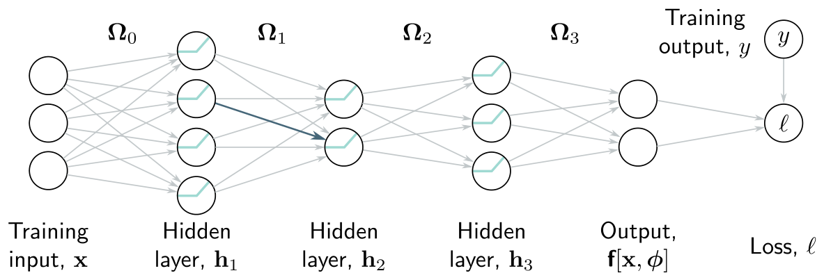
From Week 5, each training pair contributes a loss term \(\ell_i\), the negative log-likelihood of the label \(\mathbf{y}_i\) given the prediction \(\mathbf{f}[\mathbf{x}_i, \boldsymbol{\phi}]\) — for example the least squares term \(\ell_i = (\mathbf{f}[\mathbf{x}_i, \boldsymbol{\phi}] - y_i)^2\) — and the total loss is the sum
\[ L[\boldsymbol{\phi}] = \sum_{i=1}^{I} \ell_i. \tag{2}\]
From Week 6, the workhorse optimizer is SGD,
\[ \boldsymbol{\phi}_{t+1} \longleftarrow \boldsymbol{\phi}_t - \alpha \sum_{i \in \mathcal{B}_t} \frac{\partial \ell_i[\boldsymbol{\phi}_t]}{\partial \boldsymbol{\phi}}, \tag{3}\]
with learning rate \(\alpha\) and batch \(\mathcal{B}_t\). Everything else in Week 6 — momentum, Adam — consumes the same per-example gradients. So the computational task is precisely this: for every example \(i\) in the batch and every layer \(k \in \{0, 1, \ldots, K\}\), compute
\[ \frac{\partial \ell_i}{\partial \boldsymbol{\beta}_k} \qquad \text{and} \qquad \frac{\partial \ell_i}{\partial \boldsymbol{\Omega}_k}. \tag{4}\]
The first part of the chapter computes these with the backpropagation algorithm; the second part chooses the \(\boldsymbol{\Omega}_k\) and \(\boldsymbol{\beta}_k\) that training starts from, so that it is stable.
4 Computing Derivatives
Prince §7.2, pp. 97–100; figures on pp. 98–99.
The derivatives tell us how the loss changes when we nudge each parameter. The algebra that computes them is somewhat involved, so Prince starts with two observations that carry most of the intuition.
Observation 1: a weight’s effect is scaled by its source. Each weight — each element of \(\boldsymbol{\Omega}_k\) — multiplies the activation at a source hidden unit and adds the result to a destination unit in the next layer. Any small change to the weight is therefore amplified or attenuated by that source activation. In fig. 1, the blue weight is applied to the second hidden unit of layer 1; if that unit’s activation doubles, the effect of a small change to the blue weight doubles too. So to compute weight derivatives we must know the activations, which means running the network on every example in the batch and storing every hidden unit’s value. This is the forward pass, and the stored activations are exactly what the gradient computation will consume.
Observation 2: changes ripple forward, so derivatives can be reused backward. A small change in a weight or bias alters its destination unit, which alters every unit in the next layer, and the one after that, until the output and finally the loss change. So to know how a parameter affects the loss, we need to know how changes to every subsequent layer modify their successor. And those same quantities are needed again for every parameter in the same layer and in every earlier layer — so they can be computed once and reused (fig. 2):
- For a weight or bias feeding into \(\mathbf{h}_3\): we need (i) how a change in \(\mathbf{h}_3\) changes the output \(\mathbf{f}\), and (ii) how a change in \(\mathbf{f}\) changes the loss \(\ell\) (panel a).
- For a weight or bias feeding into \(\mathbf{h}_2\): (i) how \(\mathbf{h}_2\) affects \(\mathbf{h}_3\), then the same two terms as before (panel b).
- For a weight or bias feeding into \(\mathbf{h}_1\): (i) how \(\mathbf{h}_1\) affects \(\mathbf{h}_2\), (ii) how \(\mathbf{h}_2\) affects \(\mathbf{h}_3\), (iii) how \(\mathbf{h}_3\) changes the output, and (iv) how the output changes the loss (panel c).
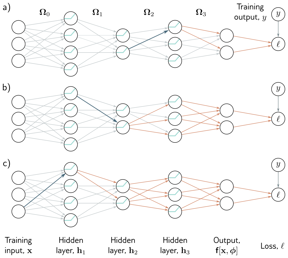
Read the list from the bottom up and every line is the previous line with one extra factor. Working backward from the loss, almost every term we need has already been computed at the previous step. Proceeding this way is the backward pass, and the reuse is the entire source of backpropagation’s efficiency.
The ideas are easy; the derivation is not, because the biases are vectors and the weights are matrices, and that requires the matrix calculus of Week 2. So, as Prince does, we first work through a model in which every quantity is a scalar.
5 A Toy Example
Prince §7.3, pp. 100–103; figures on pp. 101–103.
Consider a model with eight scalar parameters \(\boldsymbol{\phi} = \{\beta_0, \omega_0, \beta_1, \omega_1, \beta_2, \omega_2, \beta_3, \omega_3\}\) built by composing \(\sin[\bullet]\), \(\exp[\bullet]\), and \(\cos[\bullet]\):
\[ \mathrm{f}[x, \boldsymbol{\phi}] = \beta_3 + \omega_3 \cdot \cos\Big[\beta_2 + \omega_2 \cdot \exp\big[\beta_1 + \omega_1 \cdot \sin[\beta_0 + \omega_0 \cdot x]\big]\Big], \tag{5}\]
with a least squares loss \(L[\boldsymbol{\phi}] = \sum_i \ell_i\) whose terms are
\[ \ell_i = \big(\mathrm{f}[x_i, \boldsymbol{\phi}] - y_i\big)^2. \tag{6}\]
Think of it as a network with one input, one output, one hidden unit per layer, and a different activation function at each layer. We want all eight derivatives \(\partial \ell_i / \partial \beta_k\) and \(\partial \ell_i / \partial \omega_k\).
We could differentiate by hand. Here is one of the eight:
\[ \begin{aligned} \frac{\partial \ell_i}{\partial \omega_0} = \; & -2\Big(\beta_3 + \omega_3 \cos\big[\beta_2 + \omega_2 \exp[\beta_1 + \omega_1 \sin[\beta_0 + \omega_0 x_i]]\big] - y_i\Big) \cdot \omega_1 \omega_2 \omega_3 \cdot x_i \cos[\beta_0 + \omega_0 x_i] \\ & \cdot \exp\big[\beta_1 + \omega_1 \sin[\beta_0 + \omega_0 x_i]\big] \cdot \sin\Big[\beta_2 + \omega_2 \exp\big[\beta_1 + \omega_1 \sin[\beta_0 + \omega_0 x_i]\big]\Big]. \end{aligned} \tag{7}\]
Expressions like this are awkward to derive and easy to code wrongly, and they waste work: the same exponential appears three times, and most of eq. 7 reappears in the derivatives for the other seven parameters. Backpropagation computes all eight at once, in two stages.
Forward pass. Treat the loss as a chain of elementary calculations, and compute and store every intermediate value (fig. 3):
\[ \begin{aligned} f_0 &= \beta_0 + \omega_0 \cdot x_i & h_1 &= \sin[f_0] \\ f_1 &= \beta_1 + \omega_1 \cdot h_1 & h_2 &= \exp[f_1] \\ f_2 &= \beta_2 + \omega_2 \cdot h_2 & h_3 &= \cos[f_2] \\ f_3 &= \beta_3 + \omega_3 \cdot h_3 & \ell_i &= (f_3 - y_i)^2. \end{aligned} \tag{8}\]

Backward pass #1. Compute the derivatives of \(\ell_i\) with respect to the intermediate quantities, in reverse order (fig. 4). The first is direct,
\[ \frac{\partial \ell_i}{\partial f_3} = 2(f_3 - y_i), \tag{9}\]
and the next uses the chain rule,
\[ \frac{\partial \ell_i}{\partial h_3} = \frac{\partial f_3}{\partial h_3} \frac{\partial \ell_i}{\partial f_3}. \tag{10}\]
The left side asks how \(\ell_i\) changes when \(h_3\) changes. The right side decomposes that into how \(f_3\) changes when \(h_3\) changes — which is just \(\omega_3\) — times how \(\ell_i\) changes when \(f_3\) changes, which we computed one line earlier. Continuing backward,
\[ \begin{aligned} \frac{\partial \ell_i}{\partial f_2} &= \frac{\partial h_3}{\partial f_2} \left( \frac{\partial f_3}{\partial h_3} \frac{\partial \ell_i}{\partial f_3} \right) & \frac{\partial \ell_i}{\partial h_2} &= \frac{\partial f_2}{\partial h_2} \left( \frac{\partial h_3}{\partial f_2} \frac{\partial f_3}{\partial h_3} \frac{\partial \ell_i}{\partial f_3} \right) \\ \frac{\partial \ell_i}{\partial f_1} &= \frac{\partial h_2}{\partial f_1} \left( \frac{\partial f_2}{\partial h_2} \frac{\partial h_3}{\partial f_2} \frac{\partial f_3}{\partial h_3} \frac{\partial \ell_i}{\partial f_3} \right) & \frac{\partial \ell_i}{\partial h_1} &= \frac{\partial f_1}{\partial h_1} \left( \frac{\partial h_2}{\partial f_1} \frac{\partial f_2}{\partial h_2} \frac{\partial h_3}{\partial f_2} \frac{\partial f_3}{\partial h_3} \frac{\partial \ell_i}{\partial f_3} \right) \\ \frac{\partial \ell_i}{\partial f_0} &= \frac{\partial h_1}{\partial f_0} \left( \frac{\partial f_1}{\partial h_1} \frac{\partial h_2}{\partial f_1} \frac{\partial f_2}{\partial h_2} \frac{\partial h_3}{\partial f_2} \frac{\partial f_3}{\partial h_3} \frac{\partial \ell_i}{\partial f_3} \right). & & \end{aligned} \tag{11}\]
In every line the bracket was computed in the previous line, and the remaining factor is the derivative of one elementary function — a \(\cos\), an \(\exp\), a \(\sin\), or a weight. This is Observation 2 made literal.

Backward pass #2. Finally, the parameters. Each \(\beta_k\) and \(\omega_k\) enters only through \(f_k\), so one more application of the chain rule finishes the job (fig. 5):
\[ \frac{\partial \ell_i}{\partial \beta_k} = \frac{\partial f_k}{\partial \beta_k} \frac{\partial \ell_i}{\partial f_k}, \qquad \frac{\partial \ell_i}{\partial \omega_k} = \frac{\partial f_k}{\partial \omega_k} \frac{\partial \ell_i}{\partial f_k}. \tag{12}\]
The second factor in each case came from eq. 11. For \(k > 0\), \(f_k = \beta_k + \omega_k \cdot h_k\), so
\[ \frac{\partial f_k}{\partial \beta_k} = 1 \qquad \text{and} \qquad \frac{\partial f_k}{\partial \omega_k} = h_k, \tag{13}\]
which is Observation 1: the derivative with respect to a weight is proportional to its source variable \(h_k\), stored during the forward pass. For the first layer, \(f_0 = \beta_0 + \omega_0 \cdot x_i\), so
\[ \frac{\partial f_0}{\partial \beta_0} = 1 \qquad \text{and} \qquad \frac{\partial f_0}{\partial \omega_0} = x_i. \tag{14}\]

The whole procedure is a dozen lines of code. Below it is checked three ways: against the brute-force eq. 7, against finite differences, and against PyTorch.
All three agree to the precision printed. Notice also the bookkeeping: the forward pass evaluated each of \(\sin\), \(\exp\), and \(\cos\) once, and the backward pass needed each of their derivatives once — where eq. 7 alone re-evaluates the innermost exponential three times, and the other seven brute-force derivatives would repeat most of that work again.
6 The Backpropagation Algorithm
Prince §7.4, pp. 103–106; figure on p. 104.
Now the same process for the three-layer network of eq. 1. The intuition and most of the algebra carry over unchanged. What changes is that the intermediate quantities \(\mathbf{f}_k\) and \(\mathbf{h}_k\) are vectors, the biases are vectors, the weights are matrices, and the activation is a ReLU rather than \(\sin\), \(\exp\), or \(\cos\).
Forward pass. Write the network as a sequence of calculations, and store every intermediate result:
\[ \begin{aligned} \mathbf{f}_0 &= \boldsymbol{\beta}_0 + \boldsymbol{\Omega}_0 \mathbf{x}_i & \mathbf{h}_1 &= \mathbf{a}[\mathbf{f}_0] \\ \mathbf{f}_1 &= \boldsymbol{\beta}_1 + \boldsymbol{\Omega}_1 \mathbf{h}_1 & \mathbf{h}_2 &= \mathbf{a}[\mathbf{f}_1] \\ \mathbf{f}_2 &= \boldsymbol{\beta}_2 + \boldsymbol{\Omega}_2 \mathbf{h}_2 & \mathbf{h}_3 &= \mathbf{a}[\mathbf{f}_2] \\ \mathbf{f}_3 &= \boldsymbol{\beta}_3 + \boldsymbol{\Omega}_3 \mathbf{h}_3 & \ell_i &= \mathrm{l}[\mathbf{f}_3, \mathbf{y}_i]. \end{aligned} \tag{15}\]
Here \(\mathbf{f}_{k-1}\) are the pre-activations of the \(k\)th hidden layer — the values before the ReLU — and \(\mathbf{h}_k\) the activations after it. \(\mathrm{l}[\mathbf{f}_3, \mathbf{y}_i]\) is whichever Week 5 loss applies.
Backward pass #1. How does the loss change with the pre-activations? By the chain rule,
\[ \frac{\partial \ell_i}{\partial \mathbf{f}_2} = \frac{\partial \mathbf{h}_3}{\partial \mathbf{f}_2} \frac{\partial \mathbf{f}_3}{\partial \mathbf{h}_3} \frac{\partial \ell_i}{\partial \mathbf{f}_3}, \tag{16}\]
where the three factors have sizes \(D_3 \times D_3\), \(D_3 \times D_f\), and \(D_f \times 1\) for \(D_3\) hidden units in the third layer and an output of dimension \(D_f\) — the “inputs index the rows” layout of Prince’s table in Week 2. The earlier layers follow the same pattern:
\[ \begin{aligned} \frac{\partial \ell_i}{\partial \mathbf{f}_1} &= \frac{\partial \mathbf{h}_2}{\partial \mathbf{f}_1} \frac{\partial \mathbf{f}_2}{\partial \mathbf{h}_2} \left( \frac{\partial \mathbf{h}_3}{\partial \mathbf{f}_2} \frac{\partial \mathbf{f}_3}{\partial \mathbf{h}_3} \frac{\partial \ell_i}{\partial \mathbf{f}_3} \right) \\ \frac{\partial \ell_i}{\partial \mathbf{f}_0} &= \frac{\partial \mathbf{h}_1}{\partial \mathbf{f}_0} \frac{\partial \mathbf{f}_1}{\partial \mathbf{h}_1} \left( \frac{\partial \mathbf{h}_2}{\partial \mathbf{f}_1} \frac{\partial \mathbf{f}_2}{\partial \mathbf{h}_2} \frac{\partial \mathbf{h}_3}{\partial \mathbf{f}_2} \frac{\partial \mathbf{f}_3}{\partial \mathbf{h}_3} \frac{\partial \ell_i}{\partial \mathbf{f}_3} \right), \end{aligned} \tag{17}\]
and again each bracket was computed at the previous step. The individual factors are simple:
- \(\partial \ell_i / \partial \mathbf{f}_3\), the derivative of the loss with respect to the network output, depends on the loss but usually has a simple form — \(2(\mathbf{f}_3 - \mathbf{y}_i)\) for least squares.
- \(\partial \mathbf{f}_3 / \partial \mathbf{h}_3\) is the derivative of a linear map: \[ \frac{\partial \mathbf{f}_3}{\partial \mathbf{h}_3} = \frac{\partial}{\partial \mathbf{h}_3} \big(\boldsymbol{\beta}_3 + \boldsymbol{\Omega}_3 \mathbf{h}_3\big) = \boldsymbol{\Omega}_3^T, \tag{18}\] which is not obvious unless you are fluent in matrix calculus; problem 7.6 works it out, and the C7 task of Assignment A1 checked it numerically.
- \(\partial \mathbf{h}_3 / \partial \mathbf{f}_2\) depends on the activation. Each activation depends only on its own pre-activation, so the matrix is diagonal, and for a ReLU its diagonal holds a zero wherever the pre-activation was negative and a one elsewhere (fig. 6). Rather than multiply by a diagonal matrix, we extract its diagonal as the indicator vector \(\mathbb{I}[\mathbf{f}_2 > 0]\) and multiply element by element.
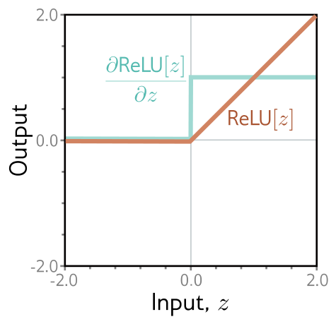
So, working back through the network, we alternately multiply by a transposed weight matrix \(\boldsymbol{\Omega}_k^T\) and mask with the indicator of which pre-activations \(\mathbf{f}_{k-1}\) were positive — both of which depend only on numbers stored in the forward pass.
Backward pass #2. The parameters. A bias enters \(\mathbf{f}_k\) additively, so
\[ \frac{\partial \ell_i}{\partial \boldsymbol{\beta}_k} = \frac{\partial \mathbf{f}_k}{\partial \boldsymbol{\beta}_k} \frac{\partial \ell_i}{\partial \mathbf{f}_k} = \frac{\partial}{\partial \boldsymbol{\beta}_k}\big(\boldsymbol{\beta}_k + \boldsymbol{\Omega}_k \mathbf{h}_k\big) \frac{\partial \ell_i}{\partial \mathbf{f}_k} = \frac{\partial \ell_i}{\partial \mathbf{f}_k}, \tag{19}\]
which backward pass #1 already produced. For the weights,
\[ \frac{\partial \ell_i}{\partial \boldsymbol{\Omega}_k} = \frac{\partial \mathbf{f}_k}{\partial \boldsymbol{\Omega}_k} \frac{\partial \ell_i}{\partial \mathbf{f}_k} = \frac{\partial}{\partial \boldsymbol{\Omega}_k}\big(\boldsymbol{\beta}_k + \boldsymbol{\Omega}_k \mathbf{h}_k\big) \frac{\partial \ell_i}{\partial \mathbf{f}_k} = \frac{\partial \ell_i}{\partial \mathbf{f}_k} \mathbf{h}_k^T. \tag{20}\]
The last step is problem 7.9, but the result is easy to sanity-check. It is an outer product, a matrix the same size as \(\boldsymbol{\Omega}_k\), linear in the activations \(\mathbf{h}_k\) that \(\boldsymbol{\Omega}_k\) multiplied — which is Observation 1 once more, in matrix form.
6.1 Backpropagation algorithm summary
Prince §7.4.1, p. 106.
For a deep network \(\mathbf{f}[\mathbf{x}_i, \boldsymbol{\phi}]\) with \(K\) hidden layers of ReLUs and loss term \(\ell_i = \mathrm{l}[\mathbf{f}[\mathbf{x}_i, \boldsymbol{\phi}], \mathbf{y}_i]\), the goal is \(\partial \ell_i / \partial \boldsymbol{\beta}_k\) and \(\partial \ell_i / \partial \boldsymbol{\Omega}_k\) for every \(k\).
Backpropagation
Forward pass. Compute and store
\[ \begin{aligned} \mathbf{f}_0 &= \boldsymbol{\beta}_0 + \boldsymbol{\Omega}_0 \mathbf{x}_i \\ \mathbf{h}_k &= \mathbf{a}[\mathbf{f}_{k-1}] & k &\in \{1, 2, \ldots, K\} \\ \mathbf{f}_k &= \boldsymbol{\beta}_k + \boldsymbol{\Omega}_k \mathbf{h}_k. & k &\in \{1, 2, \ldots, K\} \end{aligned} \tag{21}\]
Backward pass. Start from \(\partial \ell_i / \partial \mathbf{f}_K\), the derivative of the loss with respect to the network output, and work backward:
\[ \begin{aligned} \frac{\partial \ell_i}{\partial \boldsymbol{\beta}_k} &= \frac{\partial \ell_i}{\partial \mathbf{f}_k} & k &\in \{K, K-1, \ldots, 1\} \\ \frac{\partial \ell_i}{\partial \boldsymbol{\Omega}_k} &= \frac{\partial \ell_i}{\partial \mathbf{f}_k} \mathbf{h}_k^T & k &\in \{K, K-1, \ldots, 1\} \\ \frac{\partial \ell_i}{\partial \mathbf{f}_{k-1}} &= \mathbb{I}[\mathbf{f}_{k-1} > 0] \odot \left( \boldsymbol{\Omega}_k^T \frac{\partial \ell_i}{\partial \mathbf{f}_k} \right), & k &\in \{K, K-1, \ldots, 1\} \end{aligned} \tag{22}\]
where \(\odot\) is element-wise multiplication. Finish with the first layer:
\[ \frac{\partial \ell_i}{\partial \boldsymbol{\beta}_0} = \frac{\partial \ell_i}{\partial \mathbf{f}_0}, \qquad \frac{\partial \ell_i}{\partial \boldsymbol{\Omega}_0} = \frac{\partial \ell_i}{\partial \mathbf{f}_0} \mathbf{x}_i^T. \tag{23}\]
Do this for every example in the batch and sum the results to get the gradient for the SGD update, eq. 3.
Three lines in a loop, and nothing in them but matrix products, a transpose, and a mask. The cell below implements exactly eq. 21–eq. 23 in NumPy, for a whole batch at once, and compares every gradient with PyTorch’s.
loss: ours 91.3682533512   PyTorch 91.3682533512

 layer k  shape of dl/dOmega_k   max rel. error, Omega   max rel. error, beta
       0               (40, 5)                 1.9e-16                2.6e-16
       1              (40, 40)                 2.7e-16                1.8e-16
       2              (40, 40)                 3.4e-16                2.5e-16
       3               (3, 40)                 1.3e-16                1.2e-16
Agreement to machine precision, layer by layer, for gradients summed over a batch of sixteen. Two implementation details in the cell are worth copying. The sum over the batch in eq. 23 never forms sixteen separate outer products: dl_df.T @ h[k] computes their sum in one matrix product. And the indicator mask is applied by multiplying by a Boolean array, never by building the diagonal matrix fig. 6 describes.
6.2 Cheap in arithmetic, expensive in memory
Prince §7.4.1, p. 106; chapter notes, p. 114.
Prince makes two claims about the algorithm’s cost. It is extremely efficient: the most demanding step in both passes is a matrix multiplication — by \(\boldsymbol{\Omega}\) going forward, by \(\boldsymbol{\Omega}^T\) going backward — which needs only additions and multiplications. And it is not memory efficient: every intermediate value from the forward pass must be stored until the backward pass uses it, and that can limit the size of model we can train.
Both claims can be measured. For efficiency the natural comparison is the only general alternative, finite differences, which needs two forward passes per parameter.
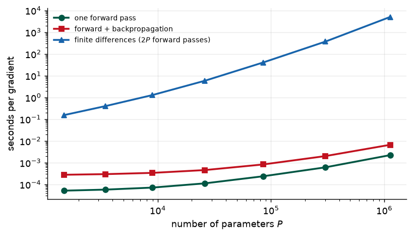
 width  parameters  forward (ms)  fwd+bwd (ms)  ratio  finite diff. (s)
    16       1,482         0.052         0.278    5.4              0.15
    32       3,466         0.058         0.297    5.1              0.40
    64       8,970         0.071         0.339    4.7              1.28
   128      26,122         0.112         0.457    4.1              5.85
   256      85,002         0.236         0.826    3.5             40.19
   512     301,066         0.608         2.002    3.3            365.98
  1024   1,126,410         2.220         6.625    3.0           5001.78
Forward plus backward costs a small, roughly constant multiple of a forward pass — typically two to four on a CPU — while finite differences get worse in proportion to the parameter count. That ratio is the precise sense in which backpropagation is “efficient”: the gradient with respect to all \(P\) parameters costs about as much as evaluating the network a few times, and independently of \(P\). It is the reason the field could scale.
Memory is the other side of the ledger. PyTorch lets us intercept every tensor it saves for the backward pass; counting those for a ten-layer network shows where the memory goes.
ten layers of Linear(256, 256) + ReLU, float32

 batch size  stored for backward (MB)   parameters (MB)   ratio
          1                      0.02              2.63     0.0
         32                      0.69              2.63     0.3
        256                      5.51              2.63     2.1
      1,024                     22.02              2.63     8.4
      4,096                     88.08              2.63    33.5
The parameters cost the same at every batch size; the stored activations grow in proportion to it, and by a batch of a thousand they already outweigh the model several times over. That is the trade the chapter notes describe. Gradient checkpointing stores only every \(N\)th layer and recomputes the rest during the backward pass, buying memory with a second forward pass (problem 7.11); micro-batching splits a batch into pieces and accumulates their gradients before stepping.
6.3 Algorithmic differentiation
Prince §7.4.2, pp. 106–107.
Understanding backpropagation matters; coding it by hand rarely does. Modern frameworks such as PyTorch and TensorFlow compute the derivatives automatically from the model specification. This is algorithmic differentiation — and, more precisely, reverse-mode algorithmic differentiation, since it accumulates the chain rule backward from the loss (problem 7.13 contrasts it with forward mode).
The design is modular. Each functional component — a linear transform, a ReLU, a loss — knows how to compute its own derivative. PyTorch’s ReLU, \(\mathbf{z}_{out} = \mathrm{relu}[\mathbf{z}_{in}]\), knows the derivative of its output with respect to its input; a linear map \(\mathbf{z}_{out} = \boldsymbol{\beta} + \boldsymbol{\Omega}\mathbf{z}_{in}\) knows its derivatives with respect to \(\mathbf{z}_{in}\), \(\boldsymbol{\beta}\), and \(\boldsymbol{\Omega}\). The framework also records the sequence of operations as the forward pass runs, so it has everything needed to run the backward pass. Both halves are visible from Python.
gradcheck of MyReLU against finite differences: True

the graph recorded during the forward pass, walked back from the loss:
SumBackward0
   PowBackward0
      AddmmBackward0
         MyReLUBackward
            AddmmBackward0
               TBackward0
gradcheck compares the hand-written backward with finite differences and passes. The printed chain is the recorded graph, walked from the loss back toward the input: a power, an affine map (AddmmBackward0), our own ReLU’s backward, another affine map. Calling .backward() on the loss runs this list in exactly that order, each node applying its own local derivative to what the node above handed it — eq. 22, assembled automatically.
These frameworks also exploit the massive parallelism of GPUs. Matrix multiplication, which dominates both passes, parallelizes naturally, and the forward and backward passes for the whole batch can run at once if the model and its stored intermediate values fit in memory. Processing the batch together means the input becomes a tensor, the generalization of a matrix to any number of dimensions: a vector is a 1D tensor, a matrix a 2D tensor. Our data so far have been vectors, so a batch has been a 2D tensor — batch index by data dimension, exactly the X_b of eq. 21’s cell. An RGB image is already 3D (height × width × channel), so a batch of them is a 4D tensor, a shape we will meet in Week 10.
6.4 Extension to arbitrary computational graphs
Prince §7.4.3, p. 107.
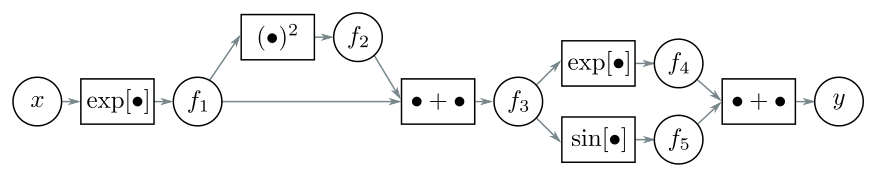
The network so far is strictly sequential: \(\mathbf{f}_0, \mathbf{h}_1, \mathbf{f}_1, \mathbf{h}_2, \ldots\) in turn. Later models branch — a hidden layer’s values might pass through two different sub-networks and be recombined. The ideas of backpropagation survive unchanged as long as the computational graph is acyclic. The one new rule is what happens where a value fans out: its derivative is the sum of the derivatives arriving back along each branch (fig. 11 in exercise 9 is a worked example). Frameworks like PyTorch handle arbitrary acyclic graphs for this reason.
autograd dl/dh          : [-2.596389  3.478013  0.386784 -1.875417]
sum of the two branches : [-2.596389  3.478013  0.386784 -1.875417]
either branch alone     : [-1.511881  1.559598  2.350996 -1.896873] (ReLU only)
7 Parameter Initialization
Prince §7.5, pp. 107–108.
Backpropagation delivers the gradients that SGD and Adam consume. Before the first gradient can be computed, the parameters need values, and this choice is far more consequential than it looks. During the forward pass each set of pre-activations is computed from the previous one as
\[ \mathbf{f}_k = \boldsymbol{\beta}_k + \boldsymbol{\Omega}_k \mathbf{h}_k = \boldsymbol{\beta}_k + \boldsymbol{\Omega}_k \mathbf{a}[\mathbf{f}_{k-1}], \tag{24}\]
with ReLU activations \(\mathbf{a}[\bullet]\). Suppose all biases start at zero and every weight is drawn from a normal distribution with mean zero and variance \(\sigma^2_\Omega\). Two scenarios bracket the problem.
- \(\sigma^2_\Omega\) very small (say \(10^{-5}\)). Each element of \(\mathbf{f}_k\) is a weighted sum of \(\mathbf{h}_k\) with tiny weights, so it is likely to be smaller in magnitude than its inputs. The ReLU then clips everything below zero, which roughly halves the range again. Layer after layer, the pre-activations shrink.
- \(\sigma^2_\Omega\) very large (say \(10^{5}\)). Each weighted sum is likely to be far larger than its inputs, and the ReLU’s halving cannot keep up. Layer after layer, the pre-activations grow.
In a deep network either trend compounds until the values cannot be represented in floating point at all. And even if the forward pass survives, the backward pass has the same structure: eq. 22 multiplies by \(\boldsymbol{\Omega}^T\) at every layer, so badly scaled weights make the gradient magnitudes shrink or grow uncontrollably as they travel back toward the input. These are the vanishing gradient problem — updates to the early layers become negligibly small — and the exploding gradient problem, in which updates become unstable.
7.1 Initialization for the forward pass
Prince §7.5.1, pp. 108–110.
Make the argument quantitative. Take two adjacent layers with pre-activations \(\mathbf{f}\) of dimension \(D_h\) and \(\mathbf{f}'\) of dimension \(D_{h'}\),
\[ \mathbf{h} = \mathbf{a}[\mathbf{f}], \qquad \mathbf{f}' = \boldsymbol{\beta} + \boldsymbol{\Omega}\mathbf{h}, \tag{25}\]
suppose each \(f_j\) has variance \(\sigma^2_f\), and initialize \(\beta_i = 0\) and \(\Omega_{ij} \sim \mathrm{Norm}[0, \sigma^2_\Omega]\). The mean of each \(f'_i\) is
\[ \mathbb{E}[f'_i] = \mathbb{E}\Big[\beta_i + \sum_{j=1}^{D_h} \Omega_{ij} h_j\Big] = \mathbb{E}[\beta_i] + \sum_{j=1}^{D_h} \mathbb{E}[\Omega_{ij}]\,\mathbb{E}[h_j] = 0 + \sum_{j=1}^{D_h} 0 \cdot \mathbb{E}[h_j] = 0, \tag{26}\]
where splitting \(\mathbb{E}[\Omega_{ij} h_j]\) into a product assumes the weights and the hidden units are independent — true at initialization, since the weights were drawn without looking at the data. Using the variance identity \(\sigma^2 = \mathbb{E}[z^2] - \mathbb{E}[z]^2\) and the same independence,
\[ \sigma^2_{f'} = \mathbb{E}[f_i'^2] - \mathbb{E}[f'_i]^2 = \mathbb{E}\Big[\Big(\sum_{j=1}^{D_h} \Omega_{ij} h_j\Big)^2\Big] = \sum_{j=1}^{D_h} \mathbb{E}[\Omega_{ij}^2]\,\mathbb{E}[h_j^2] = \sigma^2_\Omega \sum_{j=1}^{D_h} \mathbb{E}[h_j^2]. \tag{27}\]
(The cross terms vanish because distinct weights are independent with mean zero.) The ReLU enters through \(\mathbb{E}[h_j^2]\). If the pre-activations are symmetric about zero, the ReLU zeroes half of them and leaves the other half unchanged, so the second moment of \(h_j\) is half the variance of \(f_j\) (problem 7.14). Hence
\[ \sigma^2_{f'} = \sigma^2_\Omega \sum_{j=1}^{D_h} \frac{\sigma^2_f}{2} = \frac{1}{2} D_h \sigma^2_\Omega \sigma^2_f. \tag{28}\]
Every layer multiplies the variance by the same factor \(\tfrac{1}{2}D_h \sigma^2_\Omega\), so after \(K\) layers it has been multiplied by that factor to the \(K\)th power — the exponential behaviour of the two scenarios above, now with a number attached. To keep the variance constant we need the factor to be one:
\[ \sigma^2_\Omega = \frac{2}{D_h}, \tag{29}\]
where \(D_h\) is the dimension of the layer the weights are applied to. This is He initialization (He et al. 2015).
The two ingredients of eq. 28 can each be checked by sampling before we trust the conclusion.
second moment of ReLU[a] for a ~ Norm[0, sigma^2]  (problem 7.14 predicts sigma^2 / 2)
   sigma^2 =  0.5:  E[ReLU[a]^2] = 0.2497   sigma^2 / 2 = 0.2500
   sigma^2 =  1.0:  E[ReLU[a]^2] = 0.4983   sigma^2 / 2 = 0.5000
   sigma^2 =  4.0:  E[ReLU[a]^2] = 2.0001   sigma^2 / 2 = 2.0000

one layer, D_h = 100: the variance multiplier sigma^2_f' / sigma^2_f  (equation 7.30 predicts D_h sigma^2_Omega / 2)
   sigma^2_Omega = 0.001   measured   0.0487   predicted   0.0500
   sigma^2_Omega = 0.01    measured   0.4810   predicted   0.5000
   sigma^2_Omega = 0.02    measured   0.9857   predicted   1.0000
   sigma^2_Omega = 0.1     measured   5.2758   predicted   5.0000
7.2 Initialization for the backward pass
Prince §7.5.2, pp. 110–111.
The same argument applies to the gradients \(\partial \ell / \partial \mathbf{f}_k\) in the backward pass, with one change: the backward pass multiplies by the transpose \(\boldsymbol{\Omega}^T\) (eq. 22), so the sum runs over the units the weights feed into rather than the units they read from. Keeping the gradient variance constant therefore requires
\[ \sigma^2_\Omega = \frac{2}{D_{h'}}, \tag{30}\]
where \(D_{h'}\) is the dimension of the layer the weights feed into.
7.3 Initialization for both forward and backward pass
Prince §7.5.3, p. 111; figure on p. 110.
When \(\boldsymbol{\Omega}\) is square, eq. 29 and eq. 30 agree and both passes are stable together. When adjacent layers differ in width, no single variance satisfies both, and a natural compromise replaces the number of terms by the average width \((D_h + D_{h'})/2\):
\[ \sigma^2_\Omega = \frac{4}{D_h + D_{h'}}. \tag{31}\]
Fig. 8 shows what is at stake: 50 hidden layers of 100 units, a standard normal input, a target of zero with least squares loss, zero biases, and five weight variances. With He initialization, \(\sigma^2_\Omega = 2/D_h = 0.02\), the variance of the activations in the forward pass and of the gradients in the backward pass both stay level. Larger values explode and smaller values vanish, on a vertical axis that spans two hundred orders of magnitude.
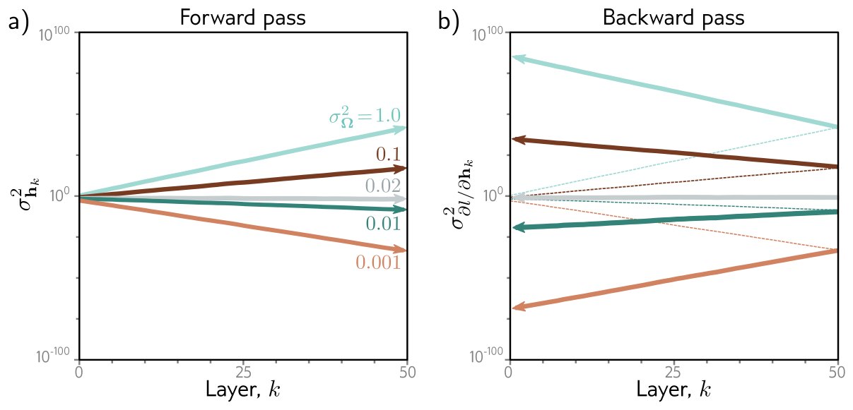
Our version runs the same experiment, overlays the prediction of eq. 28, and repeats each run over ten random draws of the weights.
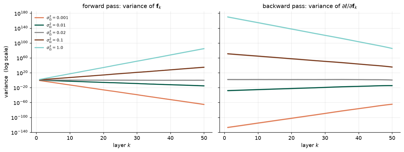
 sigma^2_Omega  factor per layer   var f_50 (median)   var dl/df_1 (median)
         0.001              0.05           5.758e-66             1.024e-127
          0.01              0.50           5.758e-16              1.024e-28
          0.02              1.00           6.483e-01              6.491e+01
           0.1              5.00           5.758e+34              1.024e+71
           1.0             50.00           5.758e+84             1.024e+170
The dashed predictions lie on top of the measured medians for every variance, so eq. 28 is not an approximation that happens to work at one setting — it is the mechanism. A factor of 0.05 per layer, which looks merely conservative, leaves \(10^{-65}\) of the signal after fifty layers; a factor of 5 produces \(10^{35}\). The backward pass doubles the damage, because the gradient at the first layer has passed through the network twice.
7.4 Initialization in practice
Ours; chapter notes, pp. 113–114.
Three practical points follow, and none of them is obvious from the derivation.
Glorot and He differ by exactly the ReLU’s factor of two. The older Glorot (or Xavier) initialization (Glorot and Bengio 2010) sets \(\sigma^2_\Omega = 2/(D_h + D_{h'})\), which is eq. 31 without the factor of two that the ReLU’s halving requires; it was derived for activations that are symmetric about zero. In a ReLU network it loses half the variance per layer — a factor of a million over twenty layers.
PyTorch does not use He initialization by default. An nn.Linear layer is initialized from a uniform distribution whose variance is \(1/(3 D_h)\), which in a ReLU network multiplies the variance by \(1/6\) per layer. This is why Prince’s training code (Section 8) calls nn.init.kaiming_normal_ explicitly.
| Scheme | \(\sigma^2_\Omega\) | Per-layer factor in a ReLU net | PyTorch |
|---|---|---|---|
| He, forward (eq. 29) | \(2/D_h\) | \(1\) | nn.init.kaiming_normal_(W) |
| He, backward (eq. 30) | \(2/D_{h'}\) | \(D_h/D_{h'}\) | nn.init.kaiming_normal_(W, mode="fan_out") |
| Prince’s compromise (eq. 31) | \(4/(D_h + D_{h'})\) | \(2D_h/(D_h + D_{h'})\) | nn.init.xavier_normal_(W, gain=2 ** 0.5) |
| Glorot / Xavier | \(2/(D_h + D_{h'})\) | \(D_h/(D_h + D_{h'})\) | nn.init.xavier_normal_(W) |
PyTorch default for nn.Linear |
\(1/(3D_h)\) | \(1/6\) | (none — it is what you get) |
The symptom of a bad initialization is a network that does not move. Below, four twenty-layer ReLU networks, identical except for how their weights were drawn, are trained on the same data with the same optimizer — SGD with momentum, the setup of Prince’s figure 7.8.
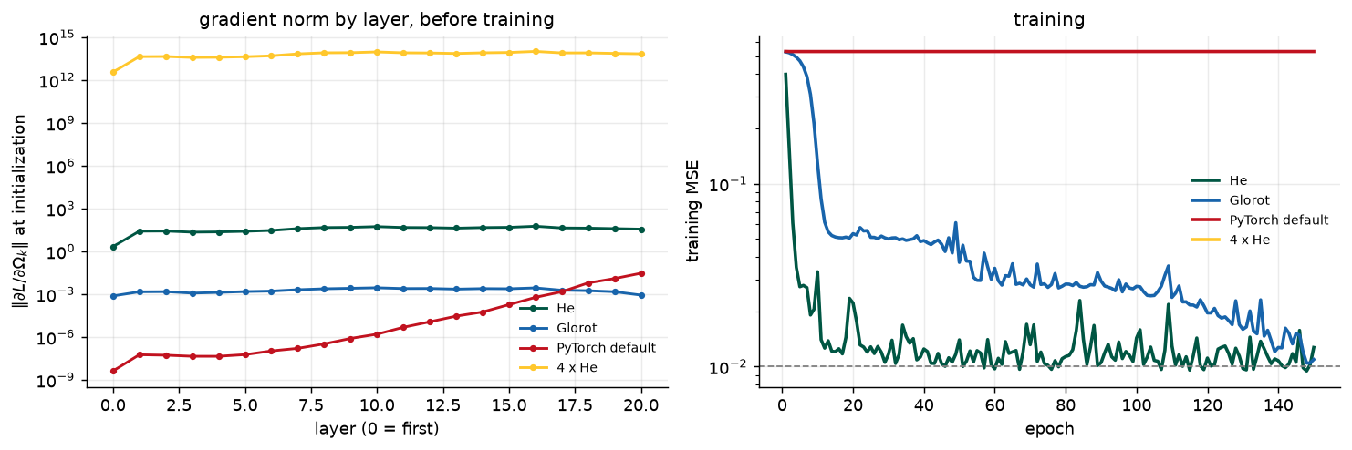
variance of the targets (loss of predicting the mean): 0.5302   noise floor: 0.0100

initialization    |grad| layer 0  |grad| last  loss ep. 5   ep. 25  ep. 150
He                      2.15e+00     3.61e+01      0.0274   0.0128   0.0127
Glorot                  7.50e-04     8.55e-04      0.4704   0.0510   0.0109
PyTorch default         4.18e-09     2.93e-02      0.5294   0.5293   0.5293
4 x He                  3.62e+12     6.92e+13         nan      nan      nan
The ordering is not an accident of one random seed: across five seeds at this learning rate, He reaches the noise floor every time, Glorot every time but several times more slowly, and the default never. One caveat cuts the other way. At a learning rate only two and a half times larger, He initialization diverged for one of the five seeds. A good initialization starts every layer with gradients of a sensible size — which also means the full step size is felt everywhere at once, and the learning rate budget is smaller than it looks.
The left panel is the diagnosis and the right the consequence. When a deep network’s loss sits at the variance of its targets — the loss of a model that predicts the mean everywhere — and refuses to move, look at the per-layer gradient norms before touching the learning rate or the architecture. If they fall by orders of magnitude toward the input, the problem is the initialization. The chapter notes list the modern alternatives — data-dependent schemes that measure the variance on a real batch, and BatchNorm, which re-normalizes at every layer during training and is a Chapter 11 topic.
8 Example Training Code
Prince §7.6, p. 111; figure on p. 112.
Prince’s book is about the ideas, not about implementation, but the code that puts this chapter and the previous two together fits on a page. Figure 7.8 is reproduced below as a listing.
import torch, torch.nn as nn
from torch.utils.data import TensorDataset, DataLoader
from torch.optim.lr_scheduler import StepLR

# define input size, hidden layer size, output size
D_i, D_k, D_o = 10, 40, 5
# create model with two hidden layers
model = nn.Sequential(
    nn.Linear(D_i, D_k),
    nn.ReLU(),
    nn.Linear(D_k, D_k),
    nn.ReLU(),
    nn.Linear(D_k, D_o))

# He initialization of weights
def weights_init(layer_in):
    if isinstance(layer_in, nn.Linear):
        nn.init.kaiming_normal_(layer_in.weight)
        layer_in.bias.data.fill_(0.0)
model.apply(weights_init)

# choose least squares loss function
criterion = nn.MSELoss()
# construct SGD optimizer and initialize learning rate and momentum
optimizer = torch.optim.SGD(model.parameters(), lr = 0.1, momentum=0.9)
# object that decreases learning rate by half every 10 epochs
scheduler = StepLR(optimizer, step_size=10, gamma=0.5)
# create 100 random data points and store in data loader class
x = torch.randn(100, D_i)
y = torch.randn(100, D_o)
data_loader = DataLoader(TensorDataset(x,y), batch_size=10, shuffle=True)

# loop over the dataset 100 times
for epoch in range(100):
    epoch_loss = 0.0
    # loop over batches
    for i, data in enumerate(data_loader):
        # retrieve inputs and labels for this batch
        x_batch, y_batch = data
        # zero the parameter gradients
        optimizer.zero_grad()
        # forward pass
        pred = model(x_batch)
        loss = criterion(pred, y_batch)
        # backward pass
        loss.backward()
        # SGD update
        optimizer.step()
        # update statistics
        epoch_loss += loss.item()
    # print error
    print(f'Epoch {epoch:5d}, loss {epoch_loss:.3f}')
    # tell scheduler to consider updating learning rate
    scheduler.step()
Every idea from Weeks 4–7 has a line here: the architecture of Week 4 (nn.Sequential), He initialization from this week (kaiming_normal_), the least squares loss of Week 5 (MSELoss), SGD with momentum and a step-decay schedule from Week 6 (SGD, StepLR), batches and epochs (DataLoader, the two loops). And all of backpropagation — every equation from eq. 15 to eq. 23 — is the single line loss.backward(). The takeaway is Prince’s: the ideas are subtle, the implementation is short.
9 Summary
Prince §7.7, pp. 111–113.
SGD needs the gradient of the loss with respect to every parameter, for every member of every batch, at every iteration, so that gradient has to be cheap. Backpropagation makes it cheap by running the network forward once, storing every pre-activation and activation, and then working backward from the loss, reusing each layer’s derivative to compute the one before it — at each step multiplying by a transposed weight matrix and masking by which ReLUs were active. The weight gradients are outer products of those backward quantities with the stored activations. The total cost is a small multiple of a forward pass regardless of the number of parameters; the price is memory, since every intermediate value must be kept until the backward pass uses it. Frameworks automate all of this by giving every operation its own derivative and recording the graph of operations as the forward pass runs, which works for any acyclic graph.
Initialization matters because each layer multiplies the variance of the activations — and, in the backward pass, of the gradients — by \(\tfrac{1}{2}D_h \sigma^2_\Omega\). Unless that factor is close to one, the activations and the gradients vanish or explode exponentially with depth, and training stalls or diverges before it starts. He initialization, \(\sigma^2_\Omega = 2/D_h\), sets the factor to exactly one for ReLU networks.
Next: we can now define a model, a loss, an optimizer, and an initialization, and train the result. What we cannot yet do is say whether the trained model is any good — whether it will perform on data it has not seen. Chapter 8 is about measuring performance: training, validation, and test error, and the surprising shape of the curve that relates them to model size.
10 Exercises
1. (UDL 7.1) A two-layer network with two hidden units per layer is \[ y = \phi_0 + \phi_1 a\big[\psi_{01} + \psi_{11} a[\theta_{01} + \theta_{11}x] + \psi_{21} a[\theta_{02} + \theta_{12}x]\big] + \phi_2 a\big[\psi_{02} + \psi_{12} a[\theta_{01} + \theta_{11}x] + \psi_{22} a[\theta_{02} + \theta_{12}x]\big], \] with ReLU activations \(a[\bullet]\), whose derivative is the indicator \(\mathbb{I}[z > 0]\). Compute the derivative of \(y\) with respect to each of the 13 parameters directly, without backpropagation. Which sub-expressions did you compute more than once? Relate your answer to Observation 2.
2. (UDL 7.2 and 7.3) Write out the final factor in each of the five chains of eq. 11 and check them against the toy-backprop cell. Then give the size of every term in eq. 17 for a network with input dimension \(D_i\), hidden widths \(D_1, D_2, D_3\), and output dimension \(D_f\).
3. (UDL 7.4 and 7.5) Compute \(\partial \ell_i / \partial \mathbf{f}[\mathbf{x}_i,
\boldsymbol{\phi}]\) — the starting point of the backward pass — for the least squares loss \(\ell_i = (y_i - \mathrm{f}[\mathbf{x}_i, \boldsymbol{\phi}])^2\) and for the binary cross-entropy \(\ell_i = -(1 - y_i)\log\big[1 - \mathrm{sig}[\mathrm{f}]\big] - y_i \log\big[\mathrm{sig}[\mathrm{f}]\big]\). The second simplifies remarkably; use it to explain why Week 5 insisted on BCEWithLogitsLoss.
4. (UDL 7.6* and 7.9*) For \(\mathbf{z} = \boldsymbol{\beta} + \boldsymbol{\Omega}\mathbf{h}\), show that \(\partial \mathbf{z} / \partial \mathbf{h} = \boldsymbol{\Omega}^T\) in Prince’s layout, by first finding \(\partial z_i / \partial h_j\). Then, for a loss \(\ell[\mathbf{f}]\) with \(\mathbf{f} = \boldsymbol{\beta} + \boldsymbol{\Omega}\mathbf{h}\), find \(\partial f_i / \partial \Omega_{ij}\) and use the chain rule to prove eq. 20.
5. (UDL 7.7 and 7.8) Compute \(\partial h / \partial f\) for the logistic sigmoid activation \(h = \mathrm{sig}[f]\). What happens to it for large positive and large negative inputs, and what does that imply for a deep network of sigmoids, given eq. 22? Then explain why the Heaviside step and the rectangular function are unusable as activations for gradient-based training.
6. (UDL 7.10*) Derive the backward pass, eq. 22, for a network with leaky ReLU activations, \(a[z] = \alpha z\) for \(z < 0\) and \(z\) otherwise. Modify backprop in the deep-backprop cell accordingly and verify it against PyTorch’s nn.LeakyReLU.
7. (UDL 7.11) A fifty-layer network fits in memory only if you store the pre-activations of every tenth layer. Explain how to compute all the derivatives using gradient checkpointing, and how much extra computation it costs. Use the saved-activations cell to estimate how much memory it saves for a batch of 4,096.
8. (UDL 7.14 and 7.15) Prove that if \(a\) is symmetric about zero with variance \(\sigma^2\), then \(\mathbb{E}[\mathrm{ReLU}[a]^2] = \sigma^2/2\), and compare with the relu-moment cell. Then: what would happen if every weight and bias were initialized to zero? Predict the answer from eq. 22, then test it by adding a fifth initialization to fig. 10.
9. (UDL 7.12* and 7.13*) For \(y = \exp\big[\exp[x] + \exp[x]^2\big] + \sin\big[\exp[x] + \exp[x]^2\big]\), with the computational graph of fig. 11, compute \(\partial y / \partial x\) by reverse-mode differentiation (in the order \(\partial y/\partial f_5, \partial y/\partial f_4, \ldots, \partial y/\partial x\)) and then by forward-mode differentiation (in the order \(\partial f_1/\partial x, \ldots, \partial y/\partial x\)). Why do we never use forward mode to compute the parameter gradients of a deep network?
10. A plant trains a 30-layer ReLU network to predict surface roughness of machined parts from 12 process variables. The loss sits at 0.84 from the first epoch and never moves; 0.84 is the variance of the measured roughness. A colleague proposes raising the learning rate tenfold. (a) Using fig. 10, explain what the loss value already tells you. (b) Which single diagnostic would you run first, and what would you expect to see? (c) The model was built with nn.Linear and no explicit initialization; compute the factor by which the pre-activation variance shrinks over 30 layers. (d) Why might raising the learning rate appear to help briefly and then fail?
11. Computational. (UDL 7.16 and 7.17) Run Prince’s training code of Section 8 and plot the loss per epoch. Then (a) remove the model.apply(weights_init) line, increase the depth to 20 hidden layers, and compare; (b) change it to a binary classification problem — binary targets, a loss from Week 5 that takes logits, and no sigmoid on the output.
12. Computational. Extend fig. 9 to activations other than the ReLU. (a) Replace ReLU by tanh and find empirically the \(\sigma^2_\Omega\) that keeps the forward variance level; compare with Glorot’s \(1/D_h\). (b) For leaky ReLU with slope \(\alpha\), derive the analogue of eq. 29 and check it against nn.init.calculate_gain("leaky_relu", alpha).
11 Textbook Reference Map
Every part of this page, mapped to Prince, Understanding Deep Learning (MIT Press, 2024) (Prince 2024). Page numbers are those of the printed book.
| This page | Prince section | Pages | Figures used |
|---|---|---|---|
| Two Problems Specific to Neural Networks | Ch. 7 opening | 96 | — |
| Problem Definitions | §7.1 | 96–97 | 7.1 (p. 98) |
| Computing Derivatives | §7.2 | 97–100 | 7.2 (p. 99) |
| A Toy Example | §7.3 | 100–103 | 7.3 (p. 101), 7.4 (p. 102), 7.5 (p. 103) |
| The Backpropagation Algorithm | §7.4 | 103–106 | 7.6 (p. 104) |
| — Backpropagation algorithm summary | §7.4.1 | 106 | — |
| — Cheap in arithmetic, expensive in memory | §7.4.1; notes | 106, 114 | — |
| — Algorithmic differentiation | §7.4.2 | 106–107 | — |
| — Extension to arbitrary computational graphs | §7.4.3 | 107 | — |
| Parameter Initialization | §7.5 | 107–108 | — |
| — Initialization for the forward pass | §7.5.1 | 108–110 | — |
| — Initialization for the backward pass | §7.5.2 | 110–111 | — |
| — Initialization for both passes | §7.5.3 | 111 | 7.7 (p. 110) |
| — Initialization in practice | ours; notes | 113–114 | — |
| Example Training Code | §7.6 | 111 | 7.8 (p. 112), as a listing |
| Summary | §7.7 | 111–113 | — |
| Exercises 1–9, 11 | Problems 7.1–7.17 | 114–117 | 7.9 (p. 116) |
Equations on this page correspond to Prince as follows: eq. 1 is his (7.1), eq. 2 is (7.2), eq. 3 is (7.3), eq. 4 is (7.4), eq. 5 is (7.5), eq. 6 is (7.6), eq. 7 is (7.7), eq. 8 is (7.8), eq. 9 is (7.10), eq. 10 is (7.11), eq. 11 is (7.12), eq. 12 is (7.13), eq. 13 is (7.14), eq. 14 is (7.15), eq. 15 is (7.16), eq. 16 is (7.17), eq. 17 is (7.18)–(7.19), eq. 18 is (7.20), eq. 19 is (7.21), eq. 20 is (7.22), eq. 21 is (7.23), eq. 22 is (7.24), eq. 23 is (7.25), eq. 24 is (7.26), eq. 25 is (7.27), eq. 26 is (7.28), eq. 27 is (7.29), eq. 28 is (7.30), eq. 29 is (7.31), eq. 30 is (7.32), and eq. 31 is (7.33). The network of exercise 1 is his (7.34) and the function of exercise 9 his (7.42).
Figure credits
Figures 7.1–7.7 and 7.9 are reproduced unaltered from Prince, Understanding Deep Learning (MIT Press, 2024), which is distributed under a Creative Commons CC-BY-NC-ND license, and are used here for non-commercial classroom instruction. Figure 7.8 is reproduced as a code listing with its contents unchanged. Figure 7.9 is adapted in the book from Domke (2010). All other figures on this page are generated by the code in this week’s notebook.
12 Further Reading
- Prince, Understanding Deep Learning, Chapter 7 (Prince 2024) — the assigned reading. The chapter notes (pp. 113–114) cover the history of backpropagation, alternative initialization schemes, memory-saving methods, and distributed training.
- ▶ UDL notebooks 7.1–7.3 — Prince’s own Colab notebooks for this chapter; links to each are at the top of this page.
- ▶ This week’s notebook — every cell above, in one Colab file.
- Rumelhart, Hinton & Williams (1986) (Rumelhart, Hinton, and Williams 1986) — the paper that named backpropagation and made networks with hidden layers trainable in practice.
- Baydin et al. (2018) (Baydin et al. 2018) — a survey of algorithmic differentiation, forward and reverse mode, written for machine learning readers.
- Glorot & Bengio (2010) (Glorot and Bengio 2010) — the variance argument for symmetric activations, and the experiments that first made vanishing gradients visible layer by layer.
- He et al. (2015) (He et al. 2015) — the factor of two for ReLUs, derived for both passes; §2.2 of the paper is eq. 27–eq. 30.
- Chen et al. (2016) (Chen et al. 2016) — gradient checkpointing, for exercise 7: memory sublinear in depth for the price of one extra forward pass.
- Ioffe & Szegedy (2015) (Ioffe and Szegedy 2015) — batch normalization, which removes most of the sensitivity to initialization and which we meet properly in Chapter 11.
References
Baydin, Atılım Güneş, Barak A. Pearlmutter, Alexey Andreyevich Radul, and Jeffrey Mark Siskind. 2018. “Automatic Differentiation in Machine Learning: A Survey.” Journal of Machine Learning Research 18 (153): 1–43.
Chen, Tianqi, Bing Xu, Chiyuan Zhang, and Carlos Guestrin. 2016. “Training Deep Nets with Sublinear Memory Cost.” arXiv Preprint arXiv:1604.06174.
Glorot, Xavier, and Yoshua Bengio. 2010. “Understanding the Difficulty of Training Deep Feedforward Neural Networks.” In International Conference on Artificial Intelligence and Statistics, 249–56.
He, Kaiming, Xiangyu Zhang, Shaoqing Ren, and Jian Sun. 2015. “Delving Deep into Rectifiers: Surpassing Human-Level Performance on ImageNet Classification.” In IEEE International Conference on Computer Vision, 1026–34.
Ioffe, Sergey, and Christian Szegedy. 2015. “Batch Normalization: Accelerating Deep Network Training by Reducing Internal Covariate Shift.” In International Conference on Machine Learning, 448–56.
Prince, Simon J. D. 2024. Understanding Deep Learning. MIT Press. https://udlbook.github.io/udlbook/.
Rumelhart, David E., Geoffrey E. Hinton, and Ronald J. Williams. 1986. “Learning Representations by Back-Propagating Errors.” Nature 323 (6088): 533–36.