Shallow Neural Networks
Week 3 · Sessions 5–6 · September 8 & 10, 2026
foundations
One hidden layer: how a stack of clipped lines becomes a piecewise linear function, why that family is universal, and what it looks like in more than one dimension and in PyTorch.
Assignment A2 — Shallow and Deep Networks
A formative notebook spanning Weeks 3 and 4: joints, activation patterns, and slopes of a shallow network; counting regions and parameters; composition, folding, and clipping; the matrix form of a deep network; and what a trained network actually realizes. Every task ends in a self-check that tells you at once whether the idea landed.
- ▶ Open A2 in Google Colab — nothing to install.
In Colab choose File → Save a copy in Drive before you start. When you are done, Runtime → Run all, then File → Download → Download .ipynb and upload that file on Blackboard under Assignment A2, named A2_<lastname>.ipynb. The deadline is posted on Blackboard.
How to read the references in these notes
Every section below opens with the section number and page range it covers in Prince, Understanding Deep Learning (MIT Press, 2024). Page numbers are those of the printed book. Figures taken from the textbook are captioned with their original figure number and page; figures generated by the code behind this page are ours. A complete cross-reference table appears in Section 12.
1 Learning Objectives
By the end of this week you should be able to:
- Write down a shallow network as an explicit equation and identify every parameter in it.
- Explain why a ReLU network computes a continuous piecewise linear function, locate the joints, and read off the slope of any region from the activation pattern.
- State the universal approximation theorem precisely, and say what it does not promise.
- Extend the model to several outputs and several inputs, and describe the geometry: shared joints, clipped planes, convex polytopes.
- Count the linear regions a shallow network can produce, and explain why that count explodes with input dimension.
- Write the general shallow network in matrix form, count its parameters, and explain why the activation must be nonlinear.
- Use the standard vocabulary (layers, units, pre-activations, weights, biases, MLP, fully connected) without hesitation.
- Implement and fit a shallow network in PyTorch, and recover its joints from the trained parameters.
The code lives in a notebook
This page shows the figures and results; the Python behind them is not printed here. All of it — every cell, in the order the note uses it — is in a notebook you can open in the browser with nothing to install:
- ▶ Open the Week 3 notebook in Google Colab — all of this page’s code, in order.
- ▶ UDL notebook 3.1 — Shallow networks I — build the ten-parameter network of eq. 1 by hand.
- ▶ UDL notebook 3.2 — Shallow networks II — two inputs and several outputs.
- ▶ UDL notebook 3.3 — Shallow network regions — count the linear regions.
- ▶ UDL notebook 3.4 — Activation functions — the alternatives to the ReLU.
Colab gives you a Python environment with NumPy, matplotlib, and PyTorch already installed. In Colab, run a cell with Shift+Enter. If you prefer to work locally, pip install -r requirements.txt from the course repository gives you the same environment.
2 Why We Need More Than a Line
Prince, Chapter 3 opening, p. 25.
Chapter 2 gave us 1D linear regression, \(y = \phi_0 + \phi_1 x\). It has two parameters and it can only ever describe a straight line. That is a severe restriction: almost nothing we care about is linear, and the cure-temperature data of Week 2 was chosen precisely because a line happened to be the right model for it.
The fix is not to abandon linear functions but to stack them around a nonlinearity. A shallow network computes several linear functions of the input, bends each one with an activation function, and then takes a linear combination of the results. That single sandwich — linear, nonlinear, linear — describes piecewise linear functions, and Prince’s claim for the chapter is that these are “expressive enough to approximate arbitrarily complex relationships between multi-dimensional inputs and outputs” (p. 25). This week shows why.
3 The Example Network
Prince §3.1, pp. 25–26; figures on p. 26.
Shallow networks are functions \(\mathbf{y} = \mathbf{f}[\mathbf{x}, \boldsymbol{\phi}]\) with parameters \(\boldsymbol{\phi}\) that map multivariate inputs to multivariate outputs. Prince defers the full definition to §3.4 and starts with the smallest interesting case: scalar input, scalar output, three hidden units, and ten parameters \(\boldsymbol{\phi} = \{\phi_0, \phi_1, \phi_2, \phi_3, \theta_{10}, \theta_{11}, \theta_{20}, \theta_{21}, \theta_{30}, \theta_{31}\}\):
\[ y = f[x, \boldsymbol{\phi}] = \phi_0 + \phi_1\, a[\theta_{10} + \theta_{11}x] + \phi_2\, a[\theta_{20} + \theta_{21}x] + \phi_3\, a[\theta_{30} + \theta_{31}x]. \tag{1}\]
Read eq. 1 in three steps:
- Compute three linear functions of the input, \(\theta_{d0} + \theta_{d1}x\) for \(d = 1, 2, 3\).
- Pass each through an activation function \(a[\cdot]\).
- Weight the three results by \(\phi_1, \phi_2, \phi_3\), sum them, and add the offset \(\phi_0\).
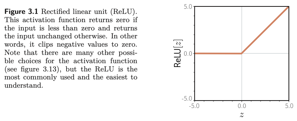
The activation function completes the description. There are many choices, but the most common is the rectified linear unit, or ReLU:
\[ a[z] = \mathrm{ReLU}[z] = \begin{cases} 0 & z < 0 \\ z & z \geq 0. \end{cases} \tag{2}\]
It returns the input when the input is positive and zero otherwise: it clips negative values to zero (fig. 1).
Notation
Following Prince, \(\theta_{d\bullet}\) are the parameters feeding into hidden unit \(d\), and \(\phi_\bullet\) are the parameters feeding out of the hidden layer into the output. The first subscript indexes the destination unit and the second the source, with \(0\) meaning the offset. Square brackets \(a[\cdot]\) denote function application, reserving parentheses for grouping.
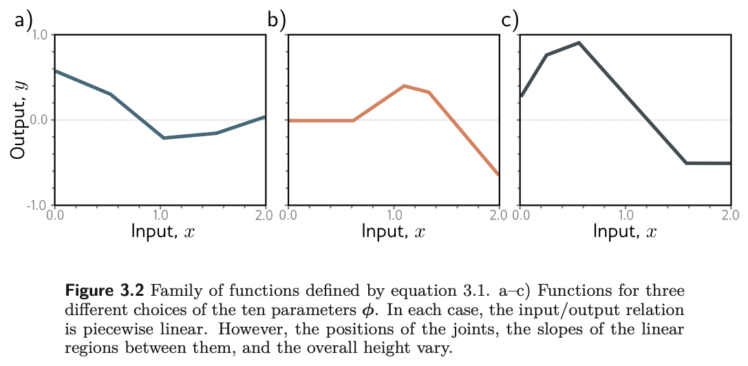
It is not obvious which family of input/output relations eq. 1 represents, and that is the question the rest of §3.1 answers. But everything from Chapter 2 already applies. The equation is a family of functions, and the ten parameters pick one member (fig. 2). Given the parameters we can perform inference by evaluating the equation at an input. Given a training set \(\{x_i, y_i\}_{i=1}^{I}\) we can define a least-squares loss \(L[\boldsymbol{\phi}]\) exactly as in Week 2, and training means searching for the \(\hat{\boldsymbol{\phi}}\) that minimizes it. Nothing about the recipe changed; only the family did.
3.1 Where the bends come from
Prince §3.1.1, pp. 26–27; figure on p. 28.
Eq. 1 represents a family of continuous piecewise linear functions with up to four linear regions. To see why, split the computation in two. First name the intermediate quantities, which Prince calls the hidden units:
Then the output is a linear function of them:
\[ y = \phi_0 + \phi_1 h_1 + \phi_2 h_2 + \phi_3 h_3. \tag{4}\]
Fig. 3 shows the flow of computation that produces the function in fig. 2a. Each hidden unit contains a line \(\theta_{\bullet 0} + \theta_{\bullet 1} x\), and the ReLU clips that line below zero. The places where the three lines cross zero become the three joints of the final output. The clipped lines are weighted by \(\phi_1, \phi_2, \phi_3\), summed, and shifted by \(\phi_0\), which controls the overall height.
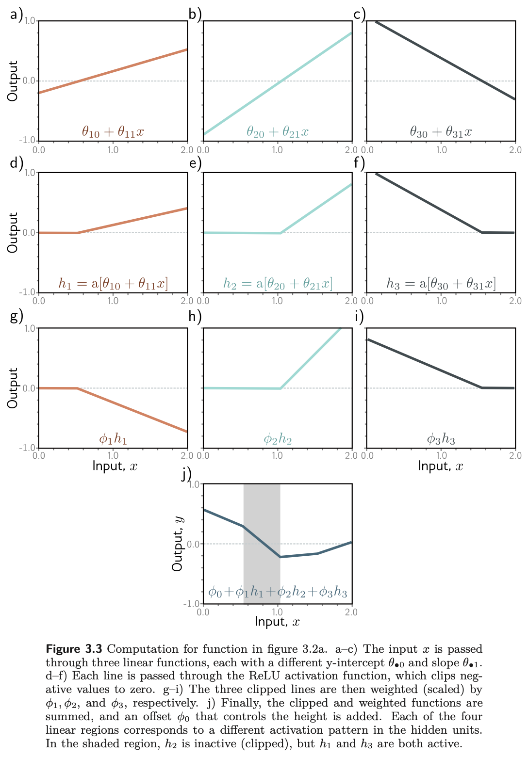
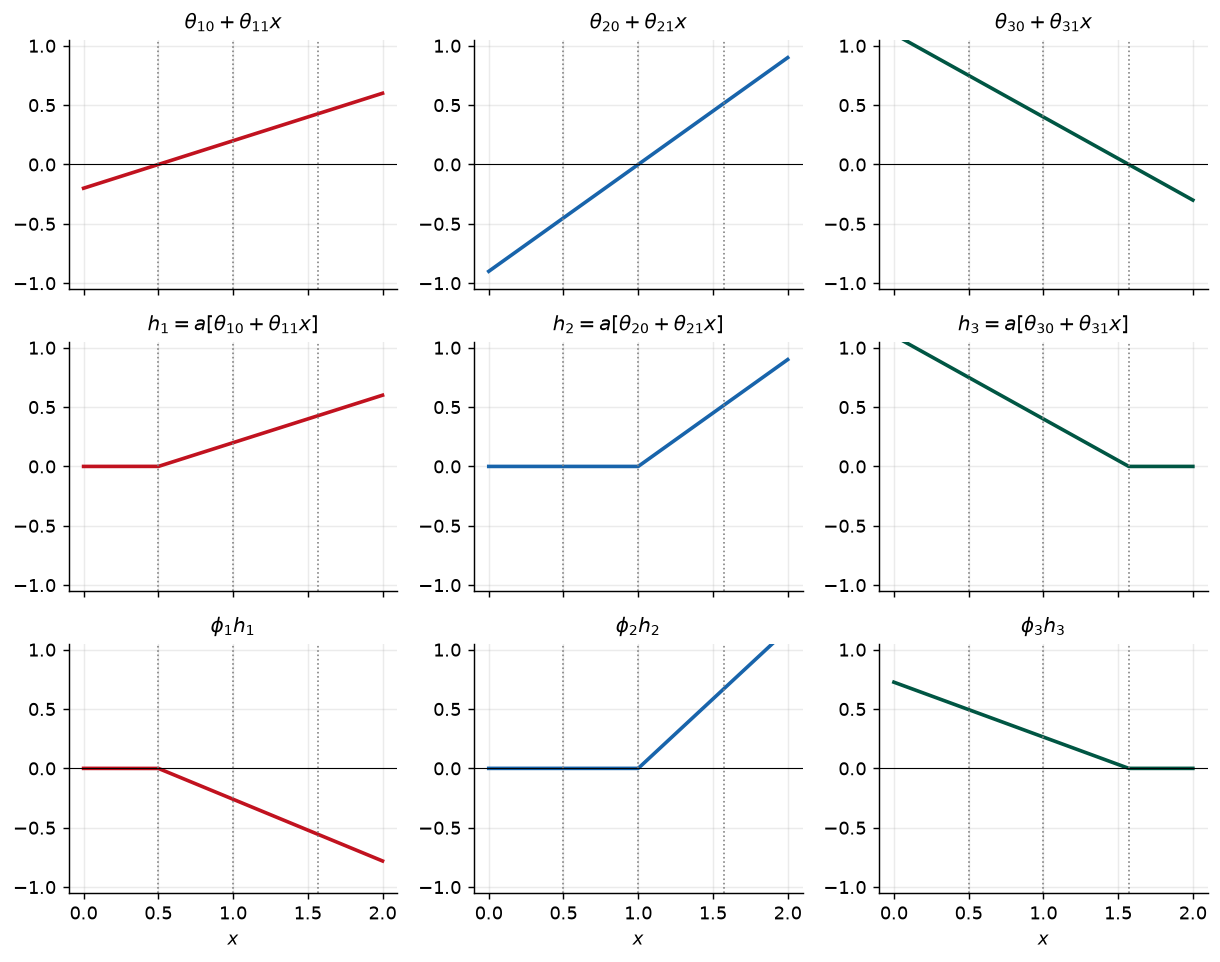
Fig. 4 is our version of the same picture, built from the exact parameters Prince gives for it in problem 3.8 (p. 40): \(\boldsymbol{\phi} = \{-0.23, -1.3, 1.3, 0.66, -0.2, 0.4, -0.9, 0.9, 1.1, -0.7\}\). Having the numbers lets us check every claim below rather than read it off a plot.
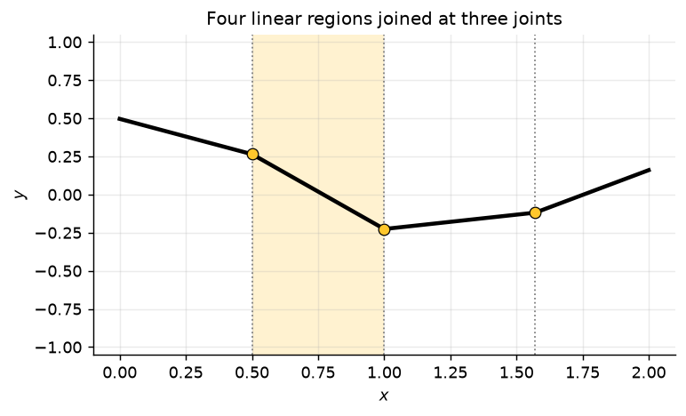
Three things to take from fig. 3, fig. 4, and fig. 5.
Each hidden unit contributes exactly one joint. Unit \(d\) bends the output where its pre-activation crosses zero, at \(x = -\theta_{d0}/\theta_{d1}\). The ReLU is linear everywhere else, so no other bends can appear. Three units give at most three joints and therefore at most four regions.
Each linear region corresponds to an activation pattern. In any region, each hidden unit is either active (not clipped) or inactive (clipped to zero), and crossing a joint flips exactly one unit. Prince’s shaded region receives contributions from \(h_1\) and \(h_3\), which are active, but not from \(h_2\), which is inactive.
The slope of a region is set by the active units. It is determined by (i) the original slopes \(\theta_{\bullet 1}\) of the active units and (ii) the weights \(\phi_\bullet\) applied to them. In the shaded region the slope is \(\theta_{11}\phi_1 + \theta_{31}\phi_3\): the slope of panel (g) of fig. 3 plus the slope of panel (i). The offset \(\phi_0\) never affects slope; it only slides the whole function up or down.
We can check that slope numerically instead of taking it on faith, and at the same time check the identity Prince poses as problem 3.9: the slope of the third region is the sum of the slopes of the first and the fourth. The activation pattern printed for each region is its signature.
region       x    active units   slope (theory)   slope (measured)
1         0.25              h3          -0.4620            -0.4620
2         0.75          h1, h3          -0.9820            -0.9820
3         1.30      h1, h2, h3           0.1880             0.1880
4         1.80          h1, h2           0.6500             0.6500

shaded region: theta_11 phi_1 + theta_31 phi_3 = -0.9820
problem 3.9  : slope(region 1) + slope(region 4) = 0.1880,  slope(region 3) = 0.1880
The last line is not a coincidence of these particular numbers. In region 3 all three units are active, in region 1 only \(h_3\) is, and in region 4 only \(h_1\) and \(h_2\) are, so the three slopes are \(\theta_{31}\phi_3\), \(\theta_{11}\phi_1 + \theta_{21}\phi_2\), and their sum.
Only three of the four slopes are free
Each hidden unit contributes one joint, so three units give four regions. But only three of the four slopes are independent: the fourth is either zero, if every unit is inactive there, or a sum of slopes from the other regions, as problem 3.9 shows. Capacity grows with hidden units, but not quite as fast as a naive count of regions suggests.
3.2 Depicting networks
Prince §3.1.2, p. 27; figure on p. 29.
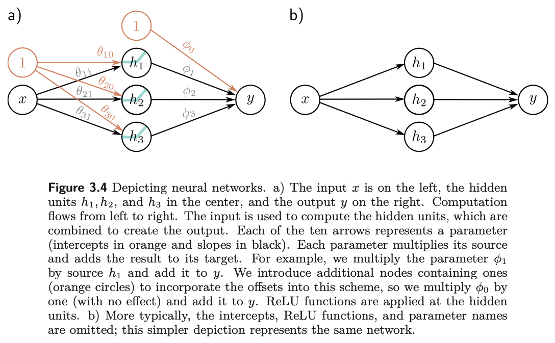
The equation and the picture are the same object. In fig. 6a the input is on the left, the three hidden units in the middle, and the output on the right, with computation flowing left to right. Each of the ten arrows is one parameter: it multiplies its source and adds the result to its target. The offsets are handled by extra nodes containing the constant one, so that \(\phi_0\) multiplies one and is added to \(y\). In practice the intercepts, the ReLU symbols, and the parameter names are all omitted, leaving the familiar circles-and-lines drawing of fig. 6b, which represents exactly the same network.
4 The Universal Approximation Theorem
Prince §3.2, pp. 29–30; figure on p. 30.
Now generalize slightly to \(D\) hidden units. The \(d\)-th hidden unit is
\[ h_d = a[\theta_{d0} + \theta_{d1}x], \tag{5}\]
and the output combines them linearly:
\[ y = \phi_0 + \sum_{d=1}^{D} \phi_d h_d. \tag{6}\]
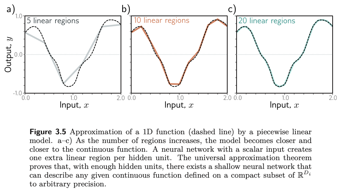
The number of hidden units is a measure of the network’s capacity. With ReLU activations the output has at most \(D\) joints, hence is piecewise linear with at most \(D + 1\) linear regions, and as we add hidden units the model can approximate more complex functions.
Indeed, with enough capacity a shallow network can describe any continuous 1D function defined on a compact subset of the real line to arbitrary precision. The argument is almost visual (fig. 7). Every hidden unit we add buys one more linear region. As the regions become more numerous each covers a shorter stretch of the input, and on a short enough stretch any continuous function is well approximated by a line.
Universal approximation theorem
For any continuous function on a compact subset of \(\mathbb{R}^{D_i}\) and any tolerance \(\epsilon > 0\), there exists a shallow network with a finite number of hidden units whose output is within \(\epsilon\) of that function everywhere on the set.
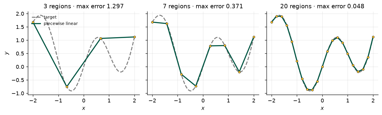
Fig. 8 repeats the experiment with a function of our own and a growing budget of regions, and prints the worst-case error each time. The models shown are piecewise linear interpolants, which are one member of the family a network with that many regions can represent; the error they achieve is therefore an upper bound on what the best such network could do.
What the theorem does not say
It is an existence result, and that is all. It does not say how many hidden units are needed, which can be astronomically many. It does not say how to find the parameters, or whether gradient descent will find them, or whether the result will generalize to data it was not fitted to. The chapter notes (p. 38) credit the theorem to Cybenko (1989) for sigmoid activations and Hornik (1991) for a much larger class. Depth, which Chapter 4 takes up, is what makes universality practical.
5 Multivariate Inputs and Outputs
Prince §3.3, pp. 30–33.
The example so far has one scalar input and one scalar output. The universal approximation theorem also holds when the network maps a multivariate input \(\mathbf{x} = [x_1, x_2, \ldots, x_{D_i}]^T\) to a multivariate output \(\mathbf{y} = [y_1, y_2, \ldots, y_{D_o}]^T\). Prince extends the model to several outputs first, then to several inputs, and only then writes the general definition.
5.1 Several outputs
Prince §3.3.1, pp. 30–31; figure on p. 31.
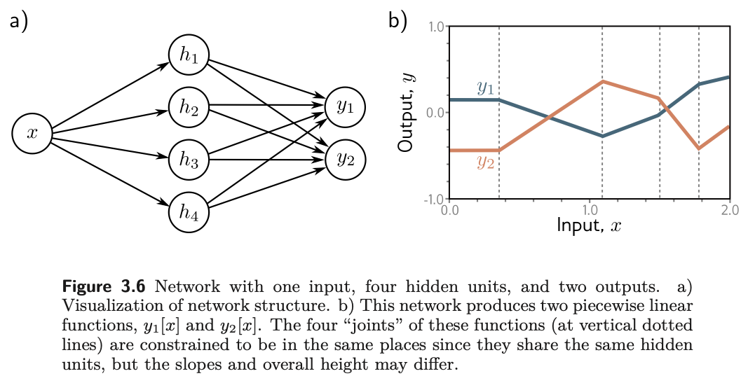
To predict several outputs, use a different linear function of the same hidden units for each. A network with a scalar input, four hidden units, and a two-dimensional output \(\mathbf{y} = [y_1, y_2]^T\) has
and
\[ \begin{aligned} y_1 &= \phi_{10} + \phi_{11}h_1 + \phi_{12}h_2 + \phi_{13}h_3 + \phi_{14}h_4 \\ y_2 &= \phi_{20} + \phi_{21}h_1 + \phi_{22}h_2 + \phi_{23}h_3 + \phi_{24}h_4. \end{aligned} \tag{8}\]
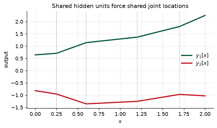
The joints in a piecewise linear output depend on where the lines \(\theta_{\bullet 0} + \theta_{\bullet 1}x\) are clipped by the ReLU at the hidden units. Because \(y_1\) and \(y_2\) are two linear functions of the same four hidden units, their four joints must be in the same places. The slopes of the regions and the overall vertical offset can differ (fig. 9).
5.2 Several inputs
Prince §3.3.2, pp. 31–33; figures on pp. 31–32.
To cope with several inputs, extend the linear relations between the input and the hidden units so that there is one slope parameter per input. A network with two inputs \(\mathbf{x} = [x_1, x_2]^T\) and a scalar output (fig. 11) might have three hidden units
combined in the usual way, \(y = \phi_0 + \phi_1 h_1 + \phi_2 h_2 + \phi_3 h_3\).
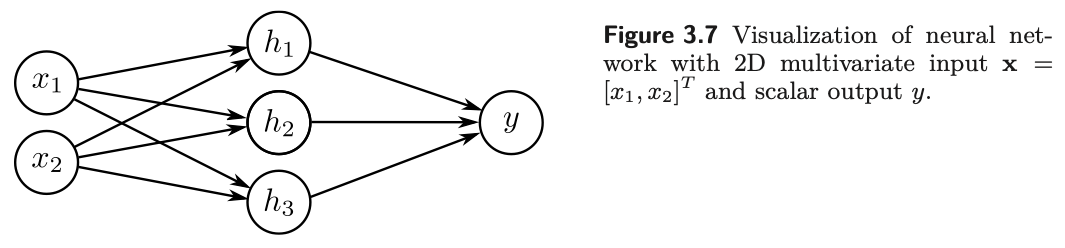
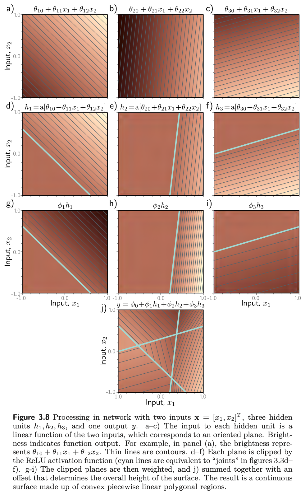
Fig. 12 shows the processing. Each hidden unit receives a linear combination of the two inputs, which is an oriented plane over the input space. The ReLU clips the negative part of each plane to zero, along the line where the plane crosses zero. The clipped planes are then recombined by the second linear function into a continuous piecewise linear surface made of convex polygonal regions, each with its own activation pattern: in the central triangle of panel (j), the first and third hidden units are active and the second is inactive.
Our version of the construction follows, with a count that the book’s figure only shows: sampling the input plane densely and tallying the distinct activation patterns gives the number of linear regions the three units carve out.
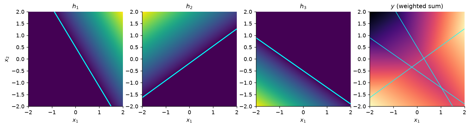
distinct activation patterns on the plane: 7
   active: none
   active: h3
   active: h2
   active: h2, h3
   active: h1
   active: h1, h3
   active: h1, h2
Three lines in general position cut the plane into seven pieces, and every piece has a different activation pattern — which is problem 3.18, done by brute force. Notice that one of the eight conceivable patterns is missing: no region has all three units active, because the three half-planes on which they are active have no common point. Regions are cells of a hyperplane arrangement, not entries in a truth table, and \(2^D\) is only an upper bound.
With more than two inputs the picture is impossible to draw but the interpretation is the same: the output is a continuous piecewise linear function of the input, and the linear regions are now convex polytopes in the multi-dimensional input space.
5.3 Regions explode with dimension
Prince §3.3.2, p. 33; figures on p. 34.
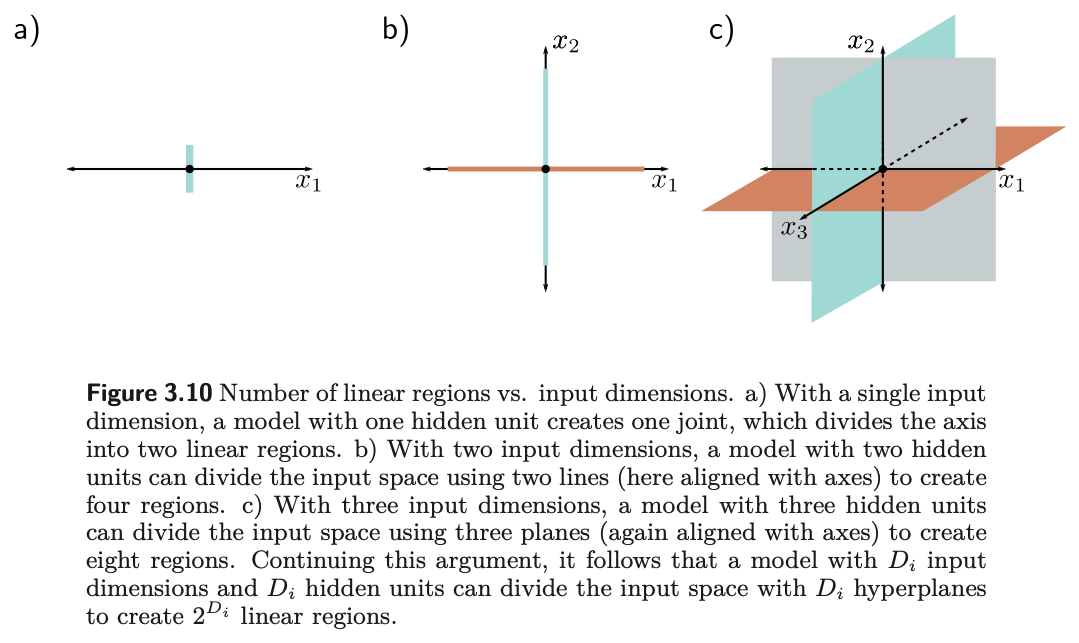
As the input dimension grows, the number of linear regions increases rapidly (fig. 14). To see how rapidly, note that each hidden unit defines a hyperplane separating the part of the input space where it is active from the part where it is not — the cyan lines of fig. 12d–f. If we had as many hidden units as input dimensions \(D_i\), we could align each hyperplane with one coordinate axis (fig. 15): two inputs give four quadrants, three give eight octants, and \(D_i\) inputs give \(2^{D_i}\) orthants. Shallow networks usually have more hidden units than input dimensions, so they create more than \(2^{D_i}\) regions.
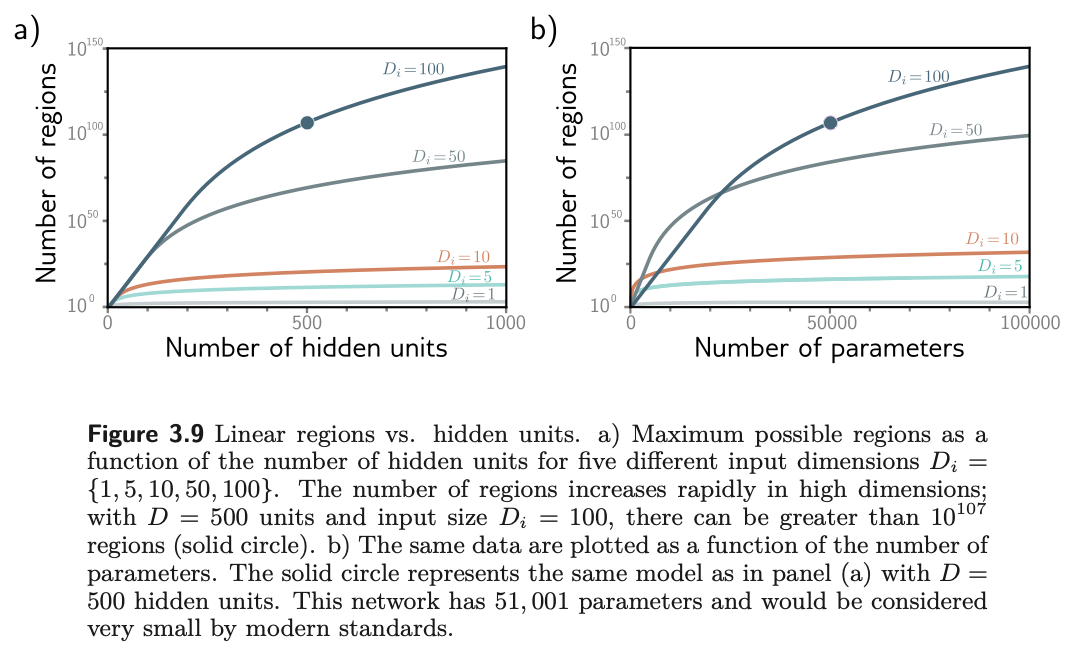
The exact maximum comes from a classical result the chapter notes cite (Zaslavsky, 1975): \(D\) hyperplanes partition a \(D_i\)-dimensional space into at most
\[ N_r = \sum_{j=0}^{D_i} \binom{D}{j} \tag{10}\]
regions. For \(D_i = 2\) and \(D = 3\) that is \(1 + 3 + 3 = 7\), the count printed above. As a rule of thumb, a shallow network with \(D > D_i\) creates somewhere between \(2^{D_i}\) and \(2^{D}\) regions. Fig. 16 evaluates eq. 10 and then puts Prince’s headline example through it.
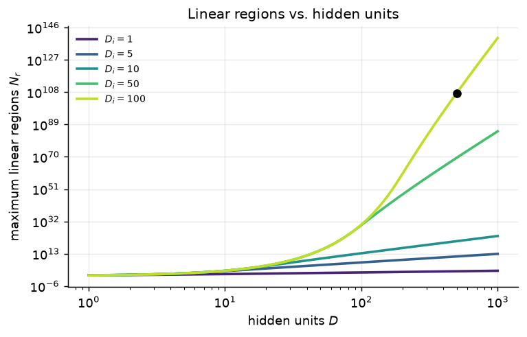
D = 500 hidden units, D_i = 100 inputs, D_o = 1 output
  parameters             : 51,001
  maximum linear regions : about 10^107
A network with 51,001 parameters is tiny by modern standards, yet it can in principle express a function with more than \(10^{107}\) distinct linear pieces (the solid circle in fig. 14 and fig. 16). Expressivity is not the bottleneck in deep learning. Finding the parameters, and having them generalize, is — which is what Chapters 6 through 9 are about.
6 The General Case
Prince §3.4, pp. 33–35; figure on p. 35.
We can now define a general shallow network \(\mathbf{y} = \mathbf{f}[\mathbf{x}, \boldsymbol{\phi}]\) that maps \(\mathbf{x} \in \mathbb{R}^{D_i}\) to \(\mathbf{y} \in \mathbb{R}^{D_o}\) through \(D\) hidden units. Each hidden unit is
and the hidden units are combined linearly to make each output:
\[ y_j = \phi_{j0} + \sum_{d=1}^{D} \phi_{jd} h_d, \tag{12}\]
where \(a[\cdot]\) is a nonlinear activation function and the parameters are \(\boldsymbol{\phi} = \{\theta_{\bullet\bullet}, \phi_{\bullet\bullet}\}\). Fig. 17 shows the case with three inputs, three hidden units, and two outputs.
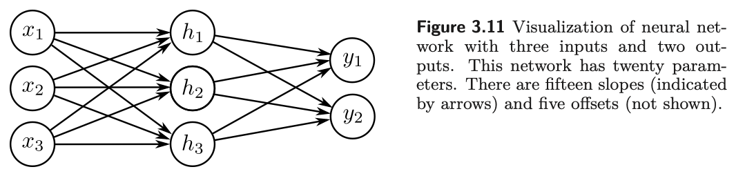
In the matrix notation of Week 2 this collapses to two lines. With \(\boldsymbol{\Theta} \in \mathbb{R}^{D \times D_i}\), \(\boldsymbol{\theta}_0 \in \mathbb{R}^{D}\), \(\boldsymbol{\Phi} \in \mathbb{R}^{D_o \times D}\), and \(\boldsymbol{\phi}_0 \in \mathbb{R}^{D_o}\),
\[ \mathbf{h} = a[\boldsymbol{\theta}_0 + \boldsymbol{\Theta}\mathbf{x}], \qquad \mathbf{y} = \boldsymbol{\phi}_0 + \boldsymbol{\Phi}\mathbf{h}, \tag{13}\]
with the activation applied elementwise. Each line is exactly the object \(\mathbf{y} = \boldsymbol{\phi}_0 + \boldsymbol{\Phi}\mathbf{z}\) that Week 2 called the most important equation in the course; a shallow network is two of them with a ReLU in between. Counting entries gives the parameter total that problem 3.17 asks for,
\[ D(D_i + 1) + D_o(D + 1), \tag{14}\]
which for fig. 17 is \(3 \cdot 4 + 2 \cdot 4 = 20\): fifteen slopes and five offsets.
The activation must be nonlinear
The activation function is what lets the model describe nonlinear relations between input and output, so it must be nonlinear itself. With no activation, or a linear one, eq. 13 becomes \(\mathbf{y} = \boldsymbol{\phi}_0 + \boldsymbol{\Phi}(\boldsymbol{\theta}_0 + \boldsymbol{\Theta}\mathbf{x})\), which is a single affine map \(\mathbf{x} \mapsto \mathbf{A}\mathbf{x} + \mathbf{b}\). The hidden layer collapses and you are back to linear regression, however many units you paid for. Problem 3.1 asks you to say this precisely.
We can confirm the collapse rather than assert it. The following builds a two-layer network with the identity in place of the ReLU, builds the single affine map it must equal, and compares them on random inputs.
two-layer network with identity activation, D = 32 hidden units
max |network output - single affine map| = 9.54e-07
The difference is floating-point noise: a two-layer linear network is a one-layer linear network, and thirty-two hidden units bought nothing.
With ReLU activations, by contrast, the network divides the input space into convex polytopes defined by the intersections of the hyperplanes at the joints of the ReLU functions. Each polytope contains a different linear function. The polytopes are the same for every output; the linear functions they contain can differ.
7 Terminology
Prince §3.5, pp. 35–36; figure on p. 36.
Neural networks come with a great deal of jargon, and Prince closes the chapter by fixing it. Fig. 18 labels the parts, and the table below is the vocabulary everything later in the course assumes.
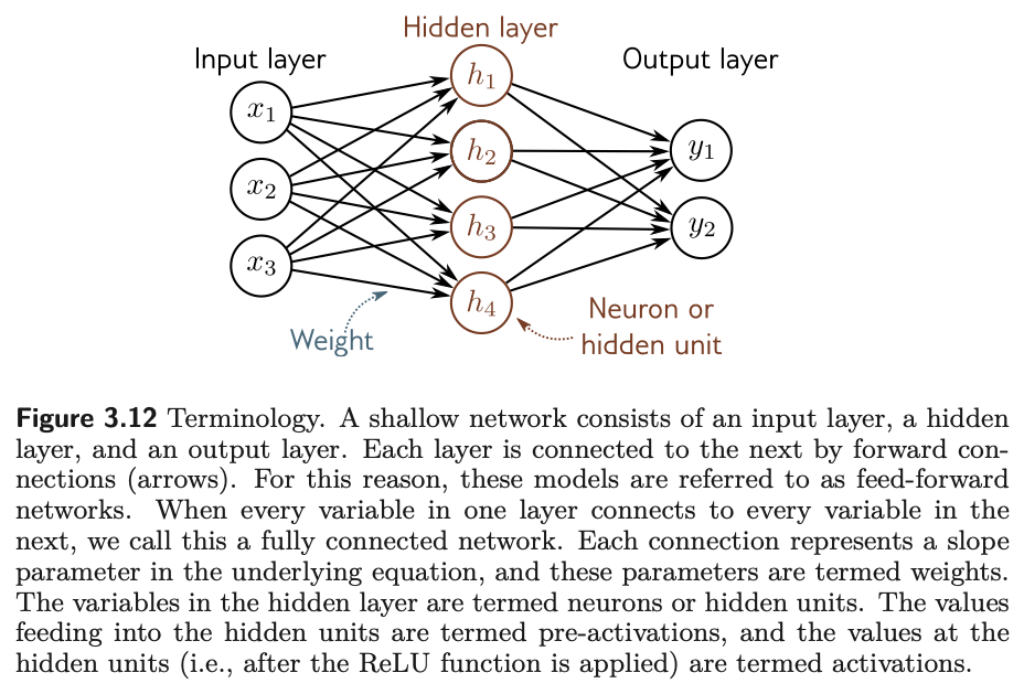
| Term | Meaning |
|---|---|
| Input layer | The inputs \(\mathbf{x}\), on the left of the diagram |
| Hidden layer | The units \(\mathbf{h}\) between input and output |
| Output layer | The predictions \(\mathbf{y}\) |
| Neuron, hidden unit | One element of \(\mathbf{h}\) |
| Pre-activation | The value fed into a hidden unit, before the ReLU |
| Activation | The value at the hidden unit, after the ReLU |
| Weights | The slope parameters, one per arrow in the diagram |
| Biases | The offset parameters \(\theta_{d0}\), \(\phi_{j0}\), not drawn |
| Multi-layer perceptron (MLP) | Any network with at least one hidden layer |
| Shallow network | Exactly one hidden layer (this chapter) |
| Deep network | More than one hidden layer (Chapter 4) |
| Feed-forward | Connections form an acyclic graph, as in every example here |
| Fully connected | Every unit in a layer connects to every unit in the next |
Why “neural”?
The chapter notes (p. 36) are candid: the models in this chapter are just functions, and the connection to biology “is, unfortunately, tenuous.” Diagrams like fig. 18 consist of densely connected nodes, which superficially resembles neurons in a brain, but there is scant evidence that brain computation works this way, and Prince advises that “it is unhelpful to think about biology going forward.” We follow that advice.
Linear, affine, and nonlinear
Strictly, a linear function obeys superposition, \(f[\mathbf{a} + \mathbf{b}] = f[\mathbf{a}] + f[\mathbf{b}]\), which the weighted sum \(\phi_1 h_1 + \phi_2 h_2 + \phi_3 h_3\) satisfies and the version with an offset \(\phi_0\) does not; the latter is properly an affine function. Machine learning conflates the two and calls both linear, and so does this course (chapter notes, p. 39). Every other function we meet is nonlinear — including the ReLU, and therefore every network that contains one.
8 Beyond the ReLU
Prince, Chapter 3 notes, pp. 37–38; figure on p. 37.
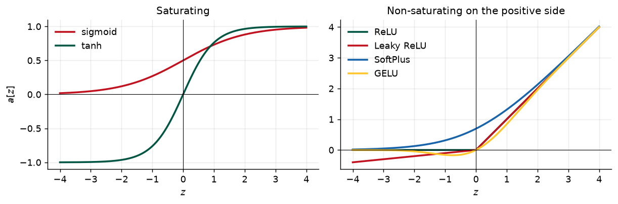
The ReLU dates back to Fukushima (1969), but in the early days the logistic sigmoid and tanh were the standard choices (fig. 19a). The ReLU was re-popularized around 2010 (Jarrett et al., 2009; Nair & Hinton, 2010; Glorot et al., 2011) and is an important part of why modern networks train at all: its derivative is exactly one for every positive input, whereas the sigmoid and tanh saturate, with derivatives near zero for large inputs of either sign. Chapter 7 makes the consequences for training precise.
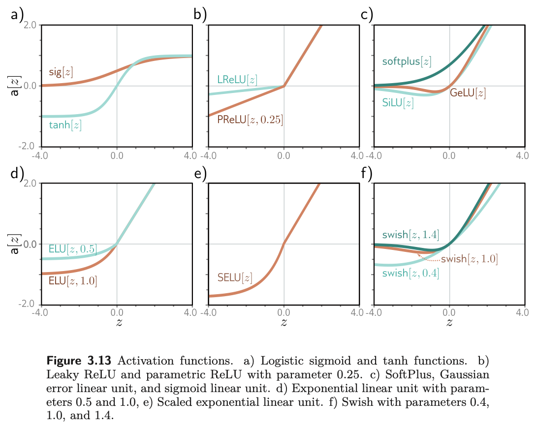
The ReLU has a flaw of its own. Its derivative is zero for negative inputs, so if every training example drives a given unit negative, the gradient with respect to that unit’s incoming weights is locally flat and training cannot “walk downhill” to fix it. This is the dying ReLU problem. Most of the alternatives in fig. 19 are attempts to resolve it while keeping the ReLU’s stable gradient on the positive side: the leaky ReLU gives the negative side a small slope of 0.1, the parametric ReLU learns that slope, and a family of smooth functions — SoftPlus, GELU, SiLU, ELU, SELU, and Swish, the last found by an automated search — round off the kink. Fig. 20 draws a handful of them in our own style.
There is no definitive winner. Prince’s verdict (p. 38) is that the leaky ReLU, the parametric ReLU, and the smooth variants give minor gains in particular situations, and he restricts the rest of the book to the plain ReLU because the functions it creates can be characterized exactly, in terms of linear regions. So do we.
9 Building One in PyTorch
Ours; UDL notebooks 3.1 and 3.3.
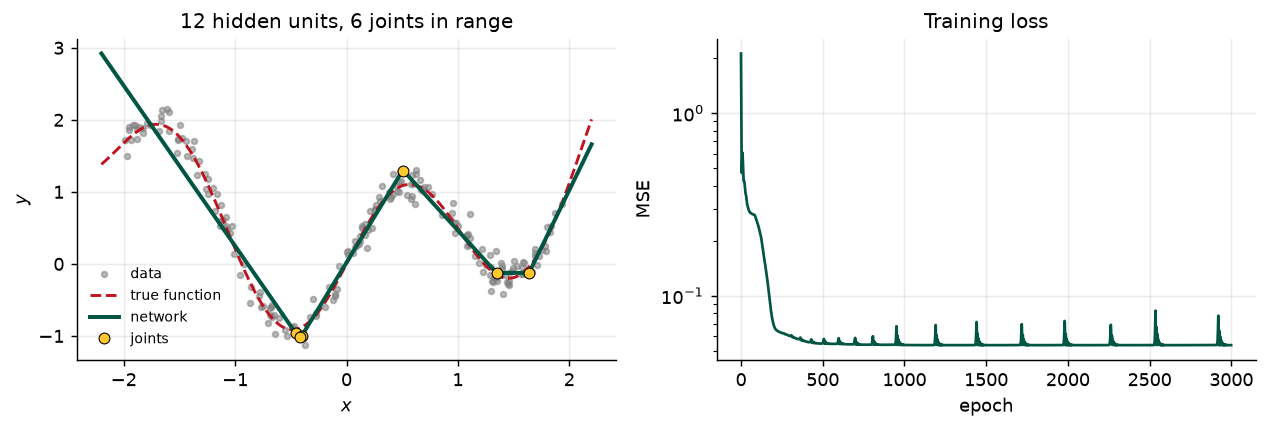
Everything above is one nn.Sequential call: a Linear layer is \(\boldsymbol{\theta}_0 + \boldsymbol{\Theta}\mathbf{x}\), a ReLU is \(a[\cdot]\), and a second Linear layer is \(\boldsymbol{\phi}_0 + \boldsymbol{\Phi}\mathbf{h}\). We fit a twelve-unit network to noisy samples of a nonlinear function and then inspect the piecewise linear structure of the trained model. The printed parameter count is eq. 14 with \(D_i = D_o = 1\).
hidden units D = 12,  parameters = 37  (formula D(Di + 1) + Do(D + 1) = 37)
final training MSE = 0.05368
Because the trained network is a shallow ReLU network, everything in §3.1 applies to it. In particular its joints sit where each hidden unit’s pre-activation crosses zero, at \(x = -\theta_{d0}/\theta_{d1}\), which we can read straight out of the first layer’s weights and biases.
9.1 Capacity in action
Ours; a preview of Prince, Chapter 8.
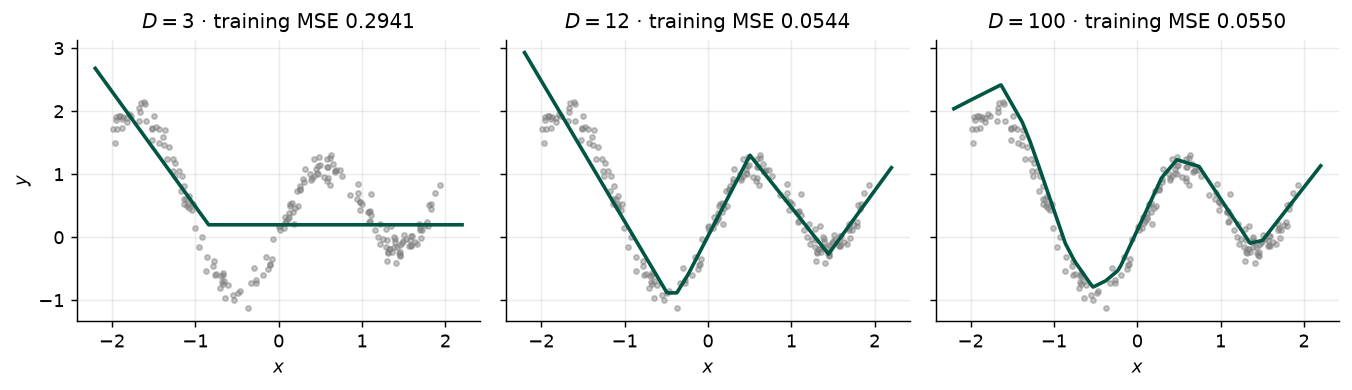
Increasing \(D\) increases the number of available regions, and with it the model’s ability to follow the data, noise included. Fig. 22 fits the same data with three, twelve, and a hundred hidden units.
10 Summary
Prince §3.6, p. 36.
Shallow neural networks have one hidden layer. They (i) compute several linear functions of the input, (ii) pass each result through an activation function, and (iii) take a linear combination of these activations to form the outputs. With ReLU activations the result is a continuous piecewise linear function: the hyperplanes defined by the hidden units carve the input space into convex polytopes, and each polytope carries its own linear function. The polytopes are shared by all the outputs; the linear functions on them are not.
Capacity is set by the number of hidden units. With enough of them a shallow network can approximate any continuous function on a compact set to arbitrary precision — but the theorem is silent on how many that takes, on how to find the parameters, and on whether they will generalize. The number of linear regions grows explosively with input dimension, so expressivity is rarely the limiting factor.
Next: Chapter 4 stacks hidden layers. The striking result is that depth buys linear regions exponentially faster than width does, which is much of why “deep” learning, rather than “wide” learning, is what took off. Chapters 5–7 then describe how these models are actually trained.
11 Exercises
1. (UDL 3.1) What kind of mapping from input to output would be created if the activation function in eq. 1 were linear, \(a[z] = \psi_0 + \psi_1 z\)? What kind would be created if the activation were removed entirely, so \(a[z] = z\)? Relate your answer to the linear-collapse check above.
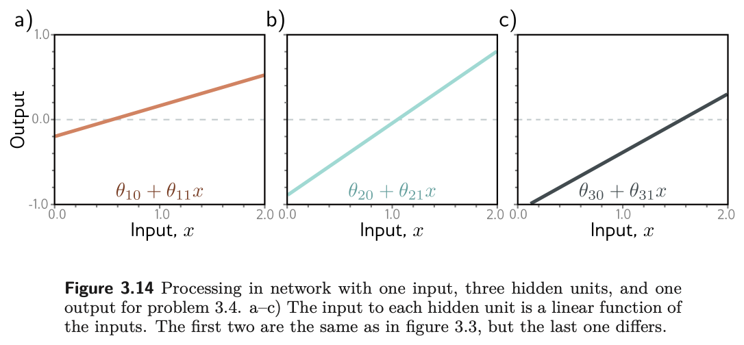
2. (UDL 3.2, 3.3*, and 3.4) For each of the four linear regions in fig. 5, state which hidden units are active and which are inactive. Then derive expressions for the positions of the three joints and for the slope of each region in terms of the ten parameters, and evaluate them with the parameters of problem 3.8 to confirm the table printed above. Finally, sketch a version of fig. 4 in which the third hidden unit’s line has changed to the one in fig. 23c, with the other parameters unchanged, and then check your sketch in the notebook.
3. (UDL 3.6) Multiply \(\theta_{10}\) and \(\theta_{11}\) by a positive constant \(\alpha\) and divide \(\phi_1\) by the same \(\alpha\). What happens to the function in eq. 1? Use the non-negative homogeneity of the ReLU, \(\mathrm{ReLU}[\alpha z] = \alpha\,\mathrm{ReLU}[z]\) for \(\alpha > 0\) (problem 3.5). What happens if \(\alpha\) is negative?
4. (UDL 3.7) Consider fitting eq. 1 with a least-squares loss. Does the loss have a unique minimum, i.e. a single “best” set of parameters? Use your answer to the previous problem, and also consider what happens when two hidden units swap roles.
5. (UDL 3.10) A network with one input, one output, and three hidden units creates up to four linear regions. Under what circumstances does it produce a function with fewer than four?
6. (UDL 3.11* and 3.17*) How many parameters does the model in fig. 9 have? Then derive eq. 14 for the general network of eq. 11 and eq. 12, and verify it in PyTorch with sum(p.numel() for p in model.parameters()) for \(D_i = 2\), \(D = 20\), \(D_o = 3\).
7. (UDL 3.15* and 3.18*) What is the maximum number of linear regions the network of fig. 17 can create? Show, using eq. 10, that the two-input, three-unit network of fig. 12 creates at most seven regions, and find the maximum when two more hidden units are added.
8. A predictive-maintenance model takes a vibration spectrum with \(D_i = 64\) frequency bins and predicts remaining useful life with a shallow network of \(D = 256\) hidden units. Write the model in the form of eq. 13 with the shape of every matrix and vector, count its parameters, and use eq. 10 to bound the number of linear regions. Then explain, in two sentences, why the “expressivity is not the bottleneck” conclusion of §3.3 applies here, and what the actual bottlenecks are likely to be for a dataset of two hundred failed bearings.
9. Computational. In the notebook, replace nn.ReLU() with nn.Sigmoid() in the PyTorch example and refit. Is the fitted function still piecewise linear? Try to locate the “joints” from the first-layer parameters as fig. 21 does, and explain what the quantity \(-\theta_{d0}/\theta_{d1}\) now means instead.
10. Computational. Fix \(D = 8\) and train the model in fig. 21 from five different random seeds. Plot the five fitted functions on one axis, with their joints. Do the joints land in the same places? Relate what you see to your answer to problem 4, and to what it implies about the loss surface that Chapter 6 will have to contend with.
12 Textbook Reference Map
Every part of this page, mapped to Prince, Understanding Deep Learning (MIT Press, 2024) (Prince 2024). Page numbers are those of the printed book.
| This page | Prince section | Pages | Figures used |
|---|---|---|---|
| Why We Need More Than a Line | Ch. 3 opening | 25 | — |
| The Example Network | §3.1 | 25–26 | 3.1, 3.2 (p. 26) |
| — Where the bends come from | §3.1.1 | 26–27 | 3.3 (p. 28) |
| — Depicting networks | §3.1.2 | 27 | 3.4 (p. 29) |
| The Universal Approximation Theorem | §3.2 | 29–30 | 3.5 (p. 30) |
| Multivariate Inputs and Outputs | §3.3 | 30 | — |
| — Several outputs | §3.3.1 | 30–31 | 3.6 (p. 31) |
| — Several inputs | §3.3.2 | 31–33 | 3.7 (p. 31), 3.8 (p. 32) |
| — Regions explode with dimension | §3.3.2 and Notes | 33, 38 | 3.9, 3.10 (p. 34) |
| The General Case | §3.4 | 33–35 | 3.11 (p. 35) |
| Terminology | §3.5 and Notes | 35–36, 39 | 3.12 (p. 36) |
| Beyond the ReLU | Notes | 37–38 | 3.13 (p. 37) |
| Building One in PyTorch | ours; notebooks 3.1, 3.3 | — | — |
| Summary | §3.6 | 36 | — |
| Exercises 1–7 | Problems 3.1–3.7, 3.10, 3.11, 3.15, 3.17, 3.18 | 39–40 | 3.14 (p. 39) |
Equations on this page correspond to Prince as follows: eq. 1 is his (3.1), eq. 2 is (3.2), eq. 3 is (3.3), eq. 4 is (3.4), eq. 5 is (3.5), eq. 6 is (3.6), eq. 7 is (3.7), eq. 8 is (3.8), eq. 9 is (3.9) together with (3.10), eq. 11 is (3.11), and eq. 12 is (3.12). eq. 13 is the matrix form of (3.11)–(3.12) in the notation of Appendix B, eq. 14 is the answer to his problem 3.17, and eq. 10 is the Zaslavsky (1975) bound quoted in the chapter notes on p. 38; none of these three appears as a numbered equation in the book.
Figure credits
Figures 3.1–3.14 are reproduced unaltered from Prince, Understanding Deep Learning (MIT Press, 2024), which is distributed under a Creative Commons CC-BY-NC-ND license, and are used here for non-commercial classroom instruction. All other figures on this page are generated by the code in this week’s notebook.
13 Further Reading
- Prince, Understanding Deep Learning, Chapter 3 (Prince 2024) — the assigned reading. The chapter notes (pp. 36–39) carry the history and the activation-function survey summarized above.
- ▶ UDL notebooks 3.1–3.4 — Prince’s own Colab notebooks for this chapter; links to each are at the top of this page.
- ▶ This week’s notebook — every cell above, in one Colab file.
- Cybenko (1989) (Cybenko 1989) and Hornik (1991) (Hornik 1991) — the original universal approximation results, for sigmoid activations and then for a general class.
- Montúfar et al. (2014) (Montúfar et al. 2014) — the counting argument for linear regions, and the reason Chapter 4 prefers depth to width.
- Nair & Hinton (2010) (Nair and Hinton 2010) — the paper that put the ReLU into the mainstream.
- Goodfellow, Bengio & Courville, Deep Learning, Chapter 6 (Goodfellow, Bengio, and Courville 2016) — a second treatment of feed-forward networks, with more on activation functions and output units.
References
Cybenko, George. 1989. “Approximation by Superpositions of a Sigmoidal Function.” Mathematics of Control, Signals and Systems 2 (4): 303–14.
Goodfellow, Ian, Yoshua Bengio, and Aaron Courville. 2016. Deep Learning. MIT Press. https://www.deeplearningbook.org/.
Hornik, Kurt. 1991. “Approximation Capabilities of Multilayer Feedforward Networks.” Neural Networks 4 (2): 251–57.
Montúfar, Guido, Razvan Pascanu, Kyunghyun Cho, and Yoshua Bengio. 2014. “On the Number of Linear Regions of Deep Neural Networks.” In Advances in Neural Information Processing Systems. Vol. 27.
Nair, Vinod, and Geoffrey E. Hinton. 2010. “Rectified Linear Units Improve Restricted Boltzmann Machines.” In International Conference on Machine Learning, 807–14.
Prince, Simon J. D. 2024. Understanding Deep Learning. MIT Press. https://udlbook.github.io/udlbook/.